Deep Learning Course · Lesson 7 of 16 · 49 min

How Networks Learn: Gradient Descent and Backpropagation

Deepak Mishra, Senior Technology Lead at Incedo

What you'll learn: how a neural network actually learns. We start by training one in four lines of PyTorch, then open the box: gradient descent, why the derivative points downhill (down to limits, continuity and Taylor's theorem), the chain rule, and backpropagation. Finally we rebuild the whole thing from scratch and check it against PyTorch.

Before you start: Lessons 1 to 6. You should know what a layer computes (a = g(Wx + b)) and recognise PyTorch's training loop. No calculus is assumed. Every piece of maths is introduced at the moment you need it.

Start with the result

Here is a complete training run. The data is the two-moons dataset: two interleaving half-circles of points that no straight line can separate. The model is a small network with one hidden layer of 16 neurons. Run it and watch the loss fall and the accuracy rise:

import torch
from torch import nn
from sklearn.datasets import make_moons

X_np, y_np = make_moons(n_samples=500, noise=0.2, random_state=0)
X = torch.tensor(X_np, dtype=torch.float32)
y = torch.tensor(y_np, dtype=torch.float32).unsqueeze(1)

torch.manual_seed(0)
model = nn.Sequential(nn.Linear(2, 16), nn.ReLU(), nn.Linear(16, 1))
loss_fn = nn.BCEWithLogitsLoss()
optimizer = torch.optim.SGD(model.parameters(), lr=0.5)

for step in range(1001):
    loss = loss_fn(model(X), y)   # 1. how wrong is the model?
    optimizer.zero_grad()         # 2. clear the gradients from the last step
    loss.backward()               # 3. backpropagation: a gradient for every weight
    optimizer.step()              # 4. gradient descent: nudge every weight downhill
    if step % 200 == 0:
        accuracy = ((model(X) > 0).float() == y).float().mean().item()
        print(f"step {step:4d}  loss {loss.item():.3f}  accuracy {accuracy:.2f}")

step    0  loss 0.680  accuracy 0.84
step  200  loss 0.240  accuracy 0.90
step  400  loss 0.151  accuracy 0.94
step  600  loss 0.106  accuracy 0.96
step  800  loss 0.091  accuracy 0.97
step 1000  loss 0.083  accuracy 0.97

The network starts with random weights. Its first loss, about 0.69, is −log ½: the loss you get by answering "50/50" for every point, so it knows essentially nothing yet. A thousand repetitions of four lines later, the loss is down to about 0.08 and the network classifies 97% of the points correctly. Everything in this lesson is about what lines 1, 3 and 4 of that loop are doing, and why it works.

What just happened

The loop repeats one idea. Line 1 measures how wrong the model is with a single number, the loss. Line 3 works out, for every weight in the network, which direction to move it to make the loss smaller; that is backpropagation. Line 4 moves every weight a small step in that direction; that is gradient descent. Repeat until the loss stops falling.

A helpful picture: imagine the loss as a hilly landscape. Your position is the current setting of all the weights, and the height is the loss. You stand in thick fog and want to reach the bottom of a valley. You can't see it, but you can feel the slope under your feet, so you take a small step downhill, feel again, and repeat. The rest of this lesson makes that picture precise.

Line 1: the loss

The loss turns "how wrong" into one number. For predicting a number (regression), the usual choice is the mean squared error. For classification it is cross-entropy, which is −log of the probability the model gave to the correct answer:

import numpy as np

for prob_of_correct_class in [0.99, 0.9, 0.5, 0.1, 0.01]:
    print(prob_of_correct_class, "-> loss", round(-np.log(prob_of_correct_class), 3))

0.99 -> loss 0.01
0.9 -> loss 0.105
0.5 -> loss 0.693
0.1 -> loss 2.303
0.01 -> loss 4.605

Being 90% sure of the right answer costs 0.105; being 1% sure costs 4.6. Confident mistakes are punished hard. (Why a logarithm, of all functions? Lesson 4 answered that: cross-entropy is the negative log-likelihood.)

Line 4: gradient descent

Gradient descent says: move each weight a little in the direction opposite to the derivative of the loss with respect to that weight. With one weight w, a learning rate η (eta) and the derivative dL/dw:

Let's watch it on the simplest possible loss, L(w) = (w − 3)², whose lowest point is at w = 3. Its derivative is dL/dw = 2(w − 3) (we'll see where that comes from shortly):

def gradient_descent(learning_rate, steps=15, w=0.0):
    for _ in range(steps):
        w = w - learning_rate * 2 * (w - 3)
    return w

for lr in [0.01, 0.1, 0.5, 0.9, 1.0, 1.1]:
    print(f"learning rate {lr}: w after 15 steps = {gradient_descent(lr):.4f}")

learning rate 0.01: w after 15 steps = 0.7843
learning rate 0.1: w after 15 steps = 2.8944
learning rate 0.5: w after 15 steps = 3.0000
learning rate 0.9: w after 15 steps = 3.1056
learning rate 1.0: w after 15 steps = 6.0000
learning rate 1.1: w after 15 steps = 49.2211

Seeing the steps makes the difference obvious. Each panel shows the loss curve in grey and the first eight values of w as dots, starting from w = 0:

PythonCopy

import numpy as np
import matplotlib.pyplot as plt

def path(learning_rate, steps=8, w=0.0):
    ws = [w]
    for _ in range(steps):
        w = w - learning_rate * 2 * (w - 3)
        ws.append(w)
    return np.array(ws)

fig, axes = plt.subplots(1, 4, figsize=(16, 3.6))
for ax, lr in zip(axes, [0.1, 0.9, 1.0, 1.1]):
    ws = path(lr)
    curve = np.linspace(min(ws.min(), 0) - 1, max(ws.max(), 6) + 1, 200)
    ax.plot(curve, (curve - 3) ** 2, color="lightgray")
    ax.plot(ws, (ws - 3) ** 2, "o-", markersize=4)
    ax.set_title(f"learning rate {lr}"); ax.set_xlabel("w")
axes[0].set_ylabel("loss (w - 3)^2")
plt.show()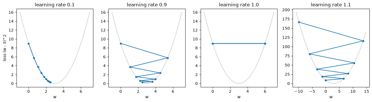

Output

A tiny learning rate crawls; a moderate one converges; 0.9 overshoots back and forth but still gets there; 1.0 bounces between 0 and 6 forever; 1.1 flies off to infinity. So it works, but only for some step sizes. A curious student should now have several questions. Why does subtracting the derivative reduce the loss at all? What is a derivative, exactly? And why does it break at exactly 1.0? The next section answers them one at a time, each answer raising the next question.

Going deeper: why does the derivative point downhill?

Question 1: why does w ← w − η·L'(w) make the loss smaller?

Zoom in far enough on any smooth curve and it looks like a straight line: its tangent. Near w, the loss is approximately the tangent line, whose slope is the derivative L'(w):

Now choose the step h = −η · L'(w), which is exactly what gradient descent does:

L'(w)² is a square, so it is never negative. Whatever the sign of the slope, the loss goes down by about η · L'(w)². If the slope is positive, we step left; if negative, we step right; either way we go downhill. That is the entire idea of gradient descent in one line. Let's check it on our example at w = 0 with η = 0.1:

L = lambda w: (w - 3) ** 2
dL = lambda w: 2 * (w - 3)

w, eta = 0.0, 0.1
actual = L(w - eta * dL(w))
predicted = L(w) - eta * dL(w) ** 2
print(f"loss before {L(w)}, after {actual:.2f}, tangent-line prediction {predicted:.2f}")

loss before 9.0, after 5.76, tangent-line prediction 5.40

The loss really did fall, from 9 to 5.76. The straight-line prediction, 5.40, is close but not exact. That gap will matter in Question 5. But first, the approximation leans entirely on the claim that a curve looks like its tangent up close. Why should that be true?

Why does a curve look like a straight line up close?

Question 2: what is the derivative, really?

Take two points on the curve, at w and at w + h. The straight line through them (a secant) has slope

Now slide the second point towards the first by making h smaller and smaller. The secant swings round and settles on the tangent. The derivative is defined as the value the secant slope settles on:

w = 0.0
for h_step in [1, 0.1, 0.01, 0.001, 0.0001]:
    secant = (L(w + h_step) - L(w)) / h_step
    print(f"h = {h_step:<7} secant slope = {secant:.4f}")

h = 1       secant slope = -5.0000
h = 0.1     secant slope = -5.9000
h = 0.01    secant slope = -5.9900
h = 0.001   secant slope = -5.9990
h = 0.0001  secant slope = -5.9999

The slopes are −5, −5.9, −5.99, −5.999, … closing in on −6, which is exactly 2(0 − 3). So the derivative is not a mysterious formula from a table; it is the slope you see when you zoom in until the curve is indistinguishable from a line. We can even do the limit by hand for this function:

That is where the formula dL/dw = 2(w − 3) came from. But the word "lim" is doing a lot of quiet work. What does "settles on" actually mean?

What does a limit mean?

Question 3: what exactly does lim (h → 0) mean?

In plain words: the limit is c if you can make the expression as close to c as you like, simply by making h small enough (but not zero, because at h = 0 the secant slope is 0/0, which is meaningless). The precise version, due to Cauchy and Weierstrass in the nineteenth century, turns "as close as you like" into a challenge and a response:

Someone challenges you with an ε: "get within 0.001 of −6". You must reply with a δ: "then keep h within this distance of 0". If you can always answer, whatever ε they pick, the limit is c. For our secant slope the reply is easy. We showed the slope is exactly −6 + h at w = 0, so its distance from −6 is just |h|. Choose δ = ε and the challenge is met every time:

def secant_slope(h_step):
    return (L(0 + h_step) - L(0)) / h_step

rng = np.random.default_rng(0)
for eps in [0.1, 0.001, 1e-6]:
    delta = eps                                       # our reply to the challenge
    hs = rng.uniform(-delta, delta, 10000)            # many h with |h| < delta
    worst = np.max(np.abs(secant_slope(hs) - (-6)))
    print(f"epsilon {eps}: worst distance from -6 = {worst:.2e}  (less than epsilon: {worst < eps})")

epsilon 0.1: worst distance from -6 = 1.00e-01  (less than epsilon: True)
epsilon 0.001: worst distance from -6 = 1.00e-03  (less than epsilon: True)
epsilon 1e-06: worst distance from -6 = 9.65e-06  (less than epsilon: False)

The first two challenges are met, but the third fails! The maths isn't wrong: the computer is. With h around a millionth, L(h) is 9.000006 and L(0) is 9, and subtracting two nearly equal floating-point numbers wipes out most of their significant digits, so the computed slope picks up rounding error larger than ε. A true limit lives in exact arithmetic, where the reply δ = ε always works; a computer can only approximate it. Keep this in mind: it is exactly why numerical derivatives later in this lesson use h around 1e-5, not 1e-12.

So the derivative exists when this game can always be won. Which raises the next question: can it always be won?

Does every function have a derivative?

Question 4: when does the limit fail, and does it matter for neural networks?

The first requirement is continuity: the function must have no jumps. Formally, f is continuous at a if the limit of f(x) as x → a equals f(a) itself. Remember the step function the perceptron used, which outputs 0 for z < 0 and 1 for z ≥ 0. It jumps at 0. Approaching from the left, the secant slope is (0 − 1)/h with h negative, which grows without bound as h shrinks. There is no tangent at a jump. Everywhere else the step function is flat, so its derivative is 0 and carries no information about which way to move. That is precisely why the perceptron could not be trained by gradient descent, and why neural networks switched to smooth activations.

Continuity is necessary, but it is not enough. The second requirement is differentiability: no sharp corners. The absolute value |x| is continuous, but at 0 the secant slope is +1 from the right and −1 from the left. Two different answers, so no single limit, so no derivative. The same happens with ReLU, max(0, x), whose one-sided slopes at 0 are 1 and 0:

relu = lambda x: np.maximum(0, x)
for name, f in [("|x|", np.abs), ("ReLU", relu)]:
    for h_step in [0.1, 0.001]:
        right = (f(0 + h_step) - f(0)) / h_step
        left = (f(0 - h_step) - f(0)) / (-h_step) + 0.0   # + 0.0 turns -0.0 into 0.0
        print(f"{name:5s} h={h_step:<6} slope from the right {right:+.1f}, from the left {left:+.1f}")

|x|   h=0.1    slope from the right +1.0, from the left -1.0
|x|   h=0.001  slope from the right +1.0, from the left -1.0
ReLU  h=0.1    slope from the right +1.0, from the left +0.0
ReLU  h=0.001  slope from the right +1.0, from the left +0.0

So the direction holds one way: every differentiable function is continuous, but not every continuous function is differentiable. The proof is one line. If the derivative exists, then

so f(a + h) → f(a), which is continuity.

But wait: almost every modern network uses ReLU, which has no derivative at 0. How can it train? Two reasons. First, the corner is a single point; the chance that a pre-activation lands on exactly 0.0 in floating point is negligible. Second, at the corner any slope between the two one-sided slopes (here, anything from 0 to 1) still describes a line that stays below the function. Such a slope is called a subgradient, and frameworks simply pick one. PyTorch picks 0:

z = torch.tensor([-1.0, 0.0, 1.0], requires_grad=True)
torch.relu(z).sum().backward()
print(z.grad)   # tensor([0., 0., 1.]): slope 0 on the left, 1 on the right, and 0 chosen at the corner

tensor([0., 0., 1.])

Why does the step size matter?

Question 5: in Question 1 the loss was only approximately the tangent line. What is the error, and is that why η = 1 broke?

Taylor's theorem gives the exact answer. For a function with a second derivative, the error of the tangent-line approximation is a squared term:

The second derivative L'' measures curvature: how quickly the slope itself changes. Substitute the gradient descent step h = −η·L'(w), and suppose the curvature is never more than some number M:

The loss is guaranteed to fall whenever the bracket is positive, that is, whenever

For L(w) = (w − 3)² the second derivative is exactly 2 everywhere, so M = 2 and the safe range is 0 < η < 1. That is precisely what the experiment showed: everything below 1 converged, 1.0 sat on the boundary and bounced forever, and 1.1 diverged. For this simple loss we can even see it exactly. Each step multiplies the distance to the minimum by a fixed factor:

This also explains the gap in Question 1: the tangent predicted 5.40, the truth was 5.76, and the difference 0.36 is exactly the Taylor term ½ · 2 · (0.6)². In a real network the curvature varies from place to place and is unknown, which is why the learning rate is tuned by experiment and why many training schedules start with a smaller learning rate and adjust it during training.

What about millions of weights?

Question 6: a real network has millions of weights. Which way is downhill then?

With many weights θ = (θ₁, …, θₙ), we take the derivative with respect to each one while holding the others fixed. These are partial derivatives, written ∂L/∂θᵢ, and together they form the gradient vector ∇L. The tangent line becomes a tangent plane (a hyperplane), with the dot product taking the place of multiplication:

Step a small distance in a direction given by a unit vector u. The loss changes at the rate ∇L · u, the directional derivative. Which direction makes it fall fastest? The Cauchy-Schwarz inequality says a dot product can never exceed the product of the lengths:

So −∇L is the steepest way down, and the multi-weight update θ ← θ − η∇L is the same rule as before, applied to every weight at once. We can test the claim by trying thousands of random directions on a two-weight loss L = x² + 10y²:

grad = np.array([2 * 1.0, 20 * 1.0])          # gradient of x^2 + 10y^2 at the point (1, 1)
angles = np.linspace(0, 2 * np.pi, 3600)
directions = np.stack([np.cos(angles), np.sin(angles)], axis=1)   # unit vectors
rates = directions @ grad                      # directional derivative in each direction

best = directions[np.argmin(rates)]
print("fastest descent found:  ", best.round(3), " rate", rates.min().round(3))
print("-gradient / |gradient|: ", (-grad / np.linalg.norm(grad)).round(3), " rate", -np.linalg.norm(grad).round(3))

fastest descent found:   [-0.1   -0.995]  rate -20.1
-gradient / |gradient|:  [-0.1   -0.995]  rate -20.1

Does gradient descent always find the best answer?

Question 7: when the gradient is zero we stop moving. Is that always the bottom?

No. ∇L = 0 at every flat point, called a critical point, and there are three kinds. A minimum curves up in every direction. A maximum curves down in every direction. A saddle point curves up in some directions and down in others, like a horse's saddle or a mountain pass. L(x, y) = x² − y² has a saddle at (0, 0). Start gradient descent exactly on the ridge and it walks into the saddle and stops; start a hair away and it escapes:

def descend(x, y, eta=0.1, steps=100):
    for _ in range(steps):
        x, y = x - eta * 2 * x, y - eta * (-2 * y)   # gradient of x^2 - y^2 is (2x, -2y)
    return x, y

print("start exactly on the ridge: ", descend(1.0, 0.0))     # stuck at the saddle (0, 0)
print("start 1e-8 off the ridge:   ", descend(1.0, 1e-8))    # y grows: it escapes

start exactly on the ridge:  (2.0370359763344877e-10, 0.0)
start 1e-8 off the ridge:    (2.0370359763344877e-10, 0.8281797452201458)

Even at a true minimum, it may be only a local minimum: the lowest point in its valley, not the lowest point overall. There is one family of functions where this can't happen. A function is convex if the straight line between any two points on its graph never dips below the graph:

A convex function is bowl-shaped, so it has no separate valleys, and every local minimum is the global minimum. Our (w − 3)² is convex. Linear and logistic regression have convex losses, which is why they always train to the same answer.

Neural network losses are not convex: they are full of saddles and separate valleys. In theory that should make training hopeless, yet it works remarkably well. In millions of dimensions, a critical point is a minimum only if the loss curves upward in every single direction, so most critical points are saddles, and the noise of mini-batch training (coming up shortly) nudges the weights off them, just as the 1e-8 did above. And research has found that in large networks most local minima have nearly the same low loss, so landing in any of them is usually fine. Why exactly this works so well is still an active research question.

That completes the ladder under line 4. We started from "why does subtracting the derivative work?" and went down through tangent lines, limits, continuity, differentiability, Taylor's theorem, gradients and convexity. Now back up to the other mysterious line: how does loss.backward() find ∂L/∂θ for every single weight?

Line 3: backpropagation

A network is a chain of simple functions: the weights produce a weighted sum z, the activation turns z into a prediction ŷ, and the loss turns ŷ into L. We know how to differentiate each link on its own. Backpropagation combines them.

Why do we multiply derivatives along a chain?

Question 8: if L depends on ŷ, which depends on z, which depends on w, how does L depend on w?

Use the tangent-line idea from Question 1 on each link. A small change Δw changes z by about (∂z/∂w)·Δw. That change in z changes ŷ by about (∂ŷ/∂z) times it, and that changes L by about (∂L/∂ŷ) times that:

Chaining linear approximations multiplies their slopes. If nudging w moves z three times as much, and z moves ŷ half as much, and ŷ moves L twice as much, then w moves L by 3 × 0.5 × 2 = 3 times as much.

You also need the derivatives of the activations, and each is a small calculation from the limit definition:

Backpropagation on one neuron, with numbers

Take one sigmoid neuron with binary cross-entropy loss: input x = 2, weight w = 0.5, bias b = 0, true label y = 1. Forward:

Backward, one link at a time. For sigmoid with cross-entropy, the first two links collapse beautifully:

def sigmoid(z):
    return 1 / (1 + np.exp(-z))

x, y_true, w, b = 2.0, 1.0, 0.5, 0.0
y_hat = sigmoid(w * x + b)
dz = y_hat - y_true
print(f"by hand:    dL/dw = {dz * x:.4f}   dL/db = {dz:.4f}")

w_t = torch.tensor(0.5, requires_grad=True)
b_t = torch.tensor(0.0, requires_grad=True)
loss = -torch.log(torch.sigmoid(w_t * 2.0 + b_t))
loss.backward()
print(f"by PyTorch: dL/dw = {w_t.grad.item():.4f}   dL/db = {b_t.grad.item():.4f}")

by hand:    dL/dw = -0.5379   dL/db = -0.2689
by PyTorch: dL/dw = -0.5379   dL/db = -0.2689

Our hand calculation and PyTorch's loss.backward() agree exactly. Backpropagation is nothing more than the chain rule, applied systematically.

What changes with many neurons?

Question 9: in a real network one weight affects the loss through many paths. How are they combined?

If a value x feeds into several values y₁, y₂, …, each of which affects L, the effects simply add up: the multivariable chain rule sums over every path.

For a whole layer these sums are exactly matrix multiplications. With a batch of m examples as rows, and each weight matrix stored as (n_in × n_out) so that Z = A_prev · W + b (PyTorch stores the transpose, as Lesson 5 showed), the backward pass for each layer is:

Two facts from linear algebra keep this manageable. First, matrix shapes must line up: an (m × n) matrix times an (n × p) matrix gives (m × p). Second, the gradient with respect to any parameter has the same shape as the parameter. If A⁽ˡ⁻¹⁾ is (m × n_in) and δ⁽ˡ⁾ is (m × n_out), then A⁽ˡ⁻¹⁾ᵀ δ⁽ˡ⁾ is (n_in × n_out), exactly the shape of W⁽ˡ⁾. Checking shapes catches most backprop bugs. The ⊙ means element-wise multiplication (NumPy's *), as opposed to matrix multiplication (NumPy's @).

Why go backwards?

Question 10: why compute the derivatives from the output backwards, rather than forwards from each weight?

Going forwards, you would track how one weight affects everything downstream, then repeat that for every weight: millions of passes for millions of weights. Going backwards, you start from the single loss value and each layer reuses the δ already computed for the layer above it. One backward pass delivers the gradient for every weight at once, at roughly the cost of one forward pass. This reverse-mode differentiation, popularised for neural networks by Rumelhart, Hinton and Williams in 1986, is what made training deep networks practical. PyTorch's autograd does exactly this: during the forward pass it records every operation in a graph, and backward() walks that graph in reverse.

Build it yourself

Now we implement the backward equations by hand in NumPy, train a network on XOR (the problem a single perceptron can't solve), and check that our gradients are identical to the ones PyTorch computes for the same weights:

X_xor = np.array([[0, 0], [0, 1], [1, 0], [1, 1]], dtype=float)
Y_xor = np.array([[0], [1], [1], [0]], dtype=float)
m = len(X_xor)

def forward_backward(W1, b1, W2, b2):
    # forward pass
    A1 = np.tanh(X_xor @ W1 + b1)
    Y_hat = sigmoid(A1 @ W2 + b2)
    loss = -np.mean(Y_xor * np.log(Y_hat) + (1 - Y_xor) * np.log(1 - Y_hat))
    # backward pass: the equations above
    dZ2 = Y_hat - Y_xor
    dW2 = A1.T @ dZ2 / m
    db2 = dZ2.mean(axis=0)
    dZ1 = (dZ2 @ W2.T) * (1 - A1 ** 2)          # tanh'(z) = 1 - tanh(z)^2
    dW1 = X_xor.T @ dZ1 / m
    db1 = dZ1.mean(axis=0)
    return loss, Y_hat, (dW1, db1, dW2, db2)

rng = np.random.default_rng(1)
params = [rng.normal(0, 1, (2, 4)), np.zeros(4), rng.normal(0, 1, (4, 1)), np.zeros(1)]

# Check against PyTorch before training
t_params = [torch.tensor(p_, requires_grad=True) for p_ in params]
A1_t = torch.tanh(torch.tensor(X_xor) @ t_params[0] + t_params[1])
Y_hat_t = torch.sigmoid(A1_t @ t_params[2] + t_params[3])
loss_t = nn.functional.binary_cross_entropy(Y_hat_t, torch.tensor(Y_xor))
loss_t.backward()
_, _, our_grads = forward_backward(*params)
print("our gradients match PyTorch:",
      all(np.allclose(g, t.grad.numpy()) for g, t in zip(our_grads, t_params)))

# Train with plain gradient descent
for epoch in range(3001):
    loss, Y_hat, grads = forward_backward(*params)
    params = [p_ - 0.5 * g for p_, g in zip(params, grads)]
    if epoch % 1000 == 0:
        print(f"epoch {epoch:4d}  loss {loss:.4f}")
print("predictions:", Y_hat.ravel().round(3))   # close to [0, 1, 1, 0]

our gradients match PyTorch: True
epoch    0  loss 0.6712
epoch 1000  loss 0.0051
epoch 2000  loss 0.0024
epoch 3000  loss 0.0016
predictions: [0.    0.998 0.998 0.003]

Checking gradients with the definition of the derivative

Question 11: if you write a new layer and its backward pass, how do you know it's right?

Go back to the definition of the derivative from Question 2 and compute it numerically: nudge one weight by a tiny h and measure the change in the loss. Use the symmetric (central) version, which is far more accurate than the one-sided one. Taylor's theorem from Question 5 shows why: in the one-sided difference the h² term leaves an error proportional to h, but in the central difference the h² terms of the two sides cancel, leaving an error proportional to h²:

f, f_prime = np.sin, np.cos                    # a function whose derivative we know exactly
for h_step in [1e-1, 1e-2, 1e-3]:
    one_sided = (f(1 + h_step) - f(1)) / h_step
    central = (f(1 + h_step) - f(1 - h_step)) / (2 * h_step)
    print(f"h={h_step:<6} one-sided error {abs(one_sided - f_prime(1)):.1e}"
          f"   central error {abs(central - f_prime(1)):.1e}")

# Gradient check on our XOR network's first weight matrix
W1 = params[0]
_, _, (dW1, _, _, _) = forward_backward(*params)
numeric = np.zeros_like(W1)
eps = 1e-5
for i in range(W1.shape[0]):
    for j in range(W1.shape[1]):
        W_plus, W_minus = W1.copy(), W1.copy()
        W_plus[i, j] += eps
        W_minus[i, j] -= eps
        loss_plus = forward_backward(W_plus, *params[1:])[0]
        loss_minus = forward_backward(W_minus, *params[1:])[0]
        numeric[i, j] = (loss_plus - loss_minus) / (2 * eps)
print("relative error:", np.linalg.norm(dW1 - numeric) / np.linalg.norm(dW1 + numeric))

h=0.1    one-sided error 4.3e-02   central error 9.0e-04
h=0.01   one-sided error 4.2e-03   central error 9.0e-06
h=0.001  one-sided error 4.2e-04   central error 9.0e-08
relative error: 6.842616022418152e-09

Each tenfold cut in h makes the one-sided error ten times smaller but the central error a hundred times smaller, exactly as the O(h) and O(h²) predict. And the gradient check agrees with our backpropagation to around a billionth.

Making it fast: mini-batches, momentum and Adam

Our loops used every example in every step (batch gradient descent). With a million examples that is far too slow per step. Mini-batch gradient descent estimates the gradient from a small random batch, typically 32 to 512 examples. The estimate is noisy, but cheap, and as Question 7 showed, the noise even helps escape saddle points. One pass through all the data is an epoch.

Plain gradient descent also zig-zags across narrow valleys (like x² + 10y², where the curvature differs by a factor of ten between directions) and crawls along flat stretches. Momentum keeps a running average of recent gradients, like a ball that builds up speed downhill and damps the zig-zag. Adam, the most common optimiser, also tracks the average squared gradient so every weight gets its own step size:

In PyTorch, switching optimiser is one line: torch.optim.Adam(model.parameters(), lr=1e-3) in place of SGD in the very first example.

Why do gradients vanish in deep networks?

Question 12: the backward pass multiplies by g'(Z) once per layer. What happens over many layers?

The derivative of the sigmoid is σ(1 − σ). A product of two numbers that add up to 1 is largest when they are equal, so σ' is at most ½ · ½ = ¼. Each sigmoid layer therefore shrinks the gradient by at least a factor of 4, and after ten layers the early weights receive less than a millionth of the signal:

s = np.linspace(0, 1, 1001)
print("largest value of s(1 - s):", (s * (1 - s)).max())          # 0.25, at s = 0.5
print("gradient factor after 10 sigmoid layers, at best:", 0.25 ** 10)

largest value of s(1 - s): 0.25
gradient factor after 10 sigmoid layers, at best: 9.5367431640625e-07

This is the vanishing gradient problem, and it held deep learning back for years. The remedies are ReLU (whose slope is exactly 1 for positive inputs), careful weight initialisation, normalisation layers, and the residual connections you'll meet with CNNs and transformers.

Summary

Training repeats four steps: compute the loss, clear the old gradients, backpropagate, and take a gradient descent step. Gradient descent works because near any point a smooth loss looks like its tangent, so stepping against the derivative lowers it by about η·L'²; the derivative is the limit of secant slopes, which exists only where the function is continuous and has no corner (ReLU's corner is handled with a subgradient). Taylor's theorem shows the step must satisfy η < 2/M for curvature M, which is exactly why large learning rates diverge. With many weights, −∇L is the steepest way down by the Cauchy-Schwarz inequality, though non-convex losses have saddles and many minima. Backpropagation is the chain rule applied backwards, layer by layer, delivering every gradient in one pass; gradient checking with central differences verifies it.

Exercises

1. Derivative by hand. Using the limit definition, show that the derivative of L(w) = w³ is 3w². Then confirm it numerically with secant slopes at w = 2.

2. Learning rate bound. For L(w) = 5(w − 1)², find the largest learning rate for which gradient descent converges. Check your answer by running gradient_descent-style code just below and just above it.

3. Continuity. Is f(x) = x · |x| differentiable at 0? Compute its one-sided secant slopes and decide. Is it continuous?

4. Steepest descent. For L(x, y) = x² + 10y² at the point (1, 1), compare one gradient descent step with η = 0.05 against a step of the same length taken straight towards the origin. Which lowers the loss more, and why doesn't the gradient point at the minimum?

5. Backpropagation. Add a second hidden layer to the NumPy XOR network, write its backward equations, and verify them with the gradient check before training.

6. Explore. In the very first PyTorch example, try learning rates of 0.05, 0.5 and 5, and swap SGD for Adam with lr=0.01. Explain what you see using Questions 5 and 7.