Deep Learning CourseLesson 6 of 16 23 min
Inside a Neural Network
What you'll learn: what is actually inside the networks you've been training. We open up a trained classifier, follow one image through it layer by layer, and then go down to the single artificial neuron and the perceptron it grew from. The questions along the way lead to the geometry of a neuron (a weight vector is perpendicular to a decision boundary), a proof that one neuron can't learn XOR, why depth needs non-linear activations, how to choose the starting weights using variances, and why a network with one hidden layer can approximate any curve.
Before you start: Lessons 1 to 5, especially dot products and lengths (Lesson 2), variance (Lesson 3) and matrices as functions (Lesson 5).
Open up a trained network
Train the Fashion-MNIST classifier from Lesson 5 again (one epoch is enough), then look inside. Every weight is an ordinary tensor you can print, and you can run an image through the layers one at a time:
import numpy as np
import torch
from torch import nn
from torch.utils.data import DataLoader
from torchvision import datasets, transforms

train_data = datasets.FashionMNIST("data", train=True, download=True, transform=transforms.ToTensor())
loader = DataLoader(train_data, batch_size=64, shuffle=True)

torch.manual_seed(0)
model = nn.Sequential(nn.Flatten(), nn.Linear(784, 128), nn.ReLU(), nn.Linear(128, 10))
optimizer = torch.optim.Adam(model.parameters(), lr=1e-3)
for images, labels in loader:                       # one epoch
    loss = nn.functional.cross_entropy(model(images), labels)
    optimizer.zero_grad(); loss.backward(); optimizer.step()

image, label = train_data[0]
x = image.unsqueeze(0)
for layer in model:
    x = layer(x)
    print(f"{layer.__class__.__name__:8s} -> shape {tuple(x.shape)}")
print("prediction:", train_data.classes[x.argmax().item()], "| truth:", train_data.classes[label])

hidden = model[2](model[1](model[0](image.unsqueeze(0))))
print(f"hidden neurons active (> 0): {(hidden > 0).sum().item()} of 128")Flatten -> shape (1, 784) Linear -> shape (1, 128) ReLU -> shape (1, 128) Linear -> shape (1, 10) prediction: Ankle boot | truth: Ankle boot hidden neurons active (> 0): 93 of 128
The image enters as 784 numbers, the first layer turns them into 128, ReLU sets the negative ones to zero (switching off 35 of the 128 neurons for this image), and the last layer turns the remaining activity into 10 class scores. Each of the 128 hidden numbers is the output of one artificial neuron. So what is a neuron?
What just happened: neurons in layers
A biological neuron receives signals from thousands of others through its dendrites, weighs them (some connections, called synapses, are strong, some weak, some inhibitory), adds them up, and fires if the total crosses a threshold. Learning, as far as neuroscience can tell, is largely the strengthening and weakening of synapses. The artificial neuron is a drastic simplification of this: multiply each input by a weight, add them up with a bias, and pass the total through an activation function g:
A layer is many neurons reading the same inputs (one row of the weight matrix each, as Lesson 5 showed), and a network is layers in sequence. The rest of this lesson builds up from a single neuron to see why this design works.
The perceptron
In 1958 Frank Rosenblatt built the perceptron: a single neuron whose activation is a step function, outputting 1 if z ≥ 0 and 0 otherwise. Choosing w₁ = w₂ = 1 and b = −1.5 makes it an AND gate, firing only when both inputs are 1; changing just the bias to −0.5 makes it an OR gate:
def perceptron(x, w, b):
    return int(np.dot(w, x) + b >= 0)

for x in [(0, 0), (0, 1), (1, 0), (1, 1)]:
print(x, "AND:", perceptron(x, [1, 1], -1.5), " OR:", perceptron(x, [1, 1], -0.5))(0, 0) AND: 0 OR: 0 (0, 1) AND: 0 OR: 1 (1, 0) AND: 0 OR: 1 (1, 1) AND: 1 OR: 1
Rosenblatt's real contribution was a rule to learn the weights from examples. Show an example, compare the prediction ŷ with the label y, and nudge the weights in proportion to the error. If the prediction was right, nothing changes; if the neuron should have fired but didn't, each weight grows in proportion to its input, and vice versa:
def train_perceptron(X, y, epochs=100, lr=0.1):
    w, b = np.zeros(X.shape[1]), 0.0
    for epoch in range(epochs):
        mistakes = 0
        for xi, target in zip(X, y):
            error = target - int(xi @ w + b >= 0)
            w, b = w + lr * error * xi, b + lr * error
            mistakes += error != 0
        if mistakes == 0:
            return w, b, f"converged after {epoch + 1} epochs"
    return w, b, f"did not converge in {epochs} epochs"

X = np.array([[0, 0], [0, 1], [1, 0], [1, 1]])
print("AND:", train_perceptron(X, np.array([0, 0, 0, 1])))
print("OR: ", train_perceptron(X, np.array([0, 1, 1, 1])))
print("XOR:", train_perceptron(X, np.array([0, 1, 1, 0])))AND: (array([0.2, 0.1]), np.float64(-0.20000000000000004), 'converged after 4 epochs') OR: (array([0.1, 0.1]), np.float64(-0.1), 'converged after 4 epochs') XOR: (array([-0.1, 0. ]), np.float64(0.0), 'did not converge in 100 epochs')
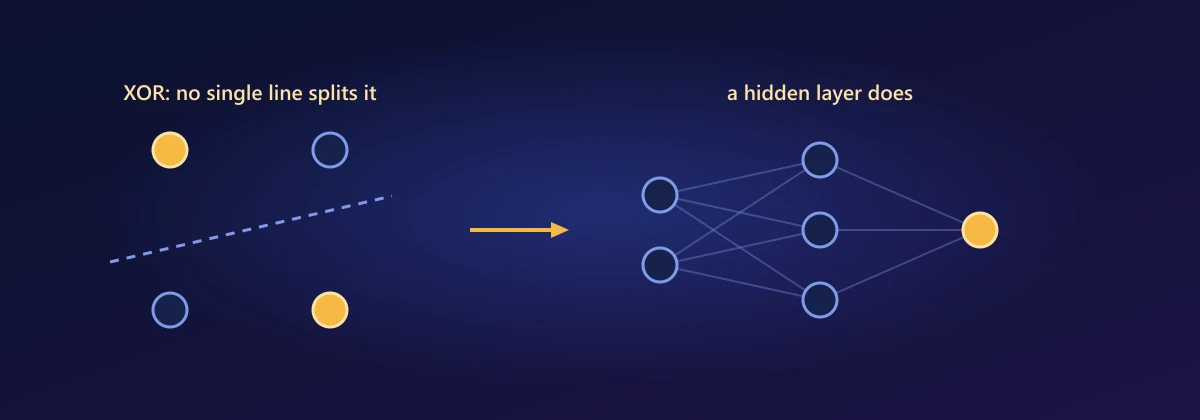
AND and OR are learned in a few epochs. XOR, which outputs 1 when exactly one input is 1, is never learned, however long we train. To see why, we need to see what a neuron does geometrically.
What shape does a neuron's decision have?
Question 1: the perceptron outputs 1 where w · x + b ≥ 0. What does that region look like?
The boundary is the set of points where w · x + b = 0. With two inputs, that's the equation of a straight line; with three, a plane; in n dimensions, a flat hyperplane. Which way does it face? Take any two points p and q on the boundary. Subtracting their equations gives w · (p − q) = 0, and Lesson 2 tells us a zero dot product means perpendicular. So w is perpendicular to every direction along the boundary: the weight vector is the boundary's normal, pointing towards the side where the neuron fires.
Even the value of z has a geometric meaning. Dividing by ‖w‖ gives the signed distance from x to the boundary:
So a neuron's pre-activation z is just the distance to its boundary, scaled by ‖w‖: positive on the firing side, negative on the other, and larger the further away the point is. Let's check with the AND neuron:
w, b = np.array([1.0, 1.0]), -1.5
on_line = [np.array([0.75, 0.75]), np.array([1.5, 0.0])]          # both satisfy x1 + x2 = 1.5
print("w is perpendicular to the boundary:", np.dot(w, on_line[0] - on_line[1]))
point = np.array([1.0, 1.0])
signed_distance = (w @ point + b) / np.linalg.norm(w)
closest = point - signed_distance * w / np.linalg.norm(w)        # step back along the normal
print("signed distance:", round(signed_distance, 4), " closest boundary point:", closest,
" which is on the line:", np.isclose(w @ closest + b, 0))w is perpendicular to the boundary: 0.0 signed distance: 0.3536 closest boundary point: [0.75 0.75] which is on the line: True
Why can't one neuron learn XOR?
Question 2: is XOR merely hard for the perceptron rule, or truly impossible for a single neuron?
It is impossible, and the proof takes four lines. XOR needs a neuron that fires for (0, 1) and (1, 0) but not for (0, 0) or (1, 1). Write out what that demands of w₁, w₂ and b:
That contradicts the last line, so no weights exist. Geometrically, the two 1s sit on one diagonal of the square and the two 0s on the other, and no straight line separates the diagonals. A single neuron can only learn linearly separable problems. Marvin Minsky and Seymour Papert made this limitation famous in 1969, and research funding for neural networks dried up for over a decade.
Multi-layer networks
The fix is to stack neurons. XOR is "OR, but not AND": XOR(x₁, x₂) = AND(OR(x₁, x₂), NAND(x₁, x₂)), and each of those is a single neuron. Two hidden neurons compute OR and NAND, and an output neuron combines them with AND:
step = lambda z: (z >= 0).astype(int)
W1 = np.array([[1, 1], [-1, -1]]); b1 = np.array([-0.5, 1.5])    # hidden: OR, NAND
W2 = np.array([[1, 1]]);           b2 = np.array([-1.5])         # output: AND

for x in X:
    hidden = step(W1 @ x + b1)
print(x, "-> hidden", hidden, "-> output", step(W2 @ hidden + b2)[0])[0 0] -> hidden [0 1] -> output 0 [0 1] -> hidden [1 1] -> output 1 [1 0] -> hidden [1 1] -> output 1 [1 1] -> hidden [1 0] -> output 0
Look at the hidden values. The four inputs become (0, 1), (1, 1), (1, 1) and (1, 0), and in that new space a single line does separate the 1s from the 0s. This is the central idea of deep learning: each layer transforms the data into a new representation in which the next layer's job is easier. Our Fashion-MNIST network does the same thing with 128 hidden neurons, learned automatically.
Why do layers need an activation function?
Question 3: what would happen if we removed the step (or ReLU) between layers?
Lesson 5 showed that applying one matrix after another is the same as applying their product. With biases the same holds, because a linear function of a linear function is linear:
A stack of any number of purely linear layers collapses into a single layer and can still only draw one flat boundary. The non-linear activation between layers is what lets depth build curved boundaries. Modern networks use smooth or nearly smooth activations rather than the step (Lesson 7 explains why the step can't be trained by gradient descent):
torch.manual_seed(0)
x = torch.randn(5, 3)
lin1, lin2 = nn.Linear(3, 4), nn.Linear(4, 2)
two_layers = lin2(lin1(x))
W_combined = lin2.weight @ lin1.weight
b_combined = lin2.weight @ lin1.bias + lin2.bias
print("two linear layers = one:", torch.allclose(two_layers, x @ W_combined.T + b_combined, atol=1e-6))
print("with ReLU between them: ", torch.allclose(lin2(torch.relu(lin1(x))), x @ W_combined.T + b_combined, atol=1e-6))two linear layers = one: True with ReLU between them: False
How big can a network's power get?
Question 4: with non-linear activations, which functions can a network represent?
Remarkably, almost all of them. Consider ReLU. One ReLU neuron, max(0, wx + b), is a hinge: flat, then a straight line from the point where wx + b = 0. Add several hinges with different positions and slopes, and you get a connected chain of straight segments, which can trace any curve as closely as you like if there are enough of them. That's the universal approximation theorem: a network with one hidden layer of enough neurons can approximate any continuous function on a bounded range to any accuracy. Watch the error fall as we give a one-hidden-layer network more hinges to fit a sine curve:
x_fit = torch.linspace(-3, 3, 400).unsqueeze(1)
y_fit = torch.sin(2 * x_fit)

for width in [2, 8, 64]:
    torch.manual_seed(0)
    net = nn.Sequential(nn.Linear(1, width), nn.ReLU(), nn.Linear(width, 1))
    opt = torch.optim.Adam(net.parameters(), lr=0.01)
    for _ in range(3000):
        loss = ((net(x_fit) - y_fit) ** 2).mean()
        opt.zero_grad(); loss.backward(); opt.step()
print(f"{width:3d} hidden neurons: mean squared error {loss.item():.5f}")2 hidden neurons: mean squared error 0.52124 8 hidden neurons: mean squared error 0.31337 64 hidden neurons: mean squared error 0.00149
The theorem guarantees that enough neurons exist, not that training will find them or that the number is reasonable. In practice, deeper networks represent complicated functions with far fewer neurons than one wide layer: each layer reuses the features of the layer before, so the number of segments can multiply with depth instead of adding.
Choosing the output layer
The final layer's activation depends on what is being predicted, and each choice pairs with the loss from Lesson 4:
| Task | Output layer | Loss |
|---|---|---|
| Regression (a price) | 1 neuron, no activation | Mean squared error |
| Binary classification | 1 neuron, sigmoid | Binary cross-entropy |
| One of K classes | K neurons, softmax | Categorical cross-entropy |
In PyTorch the sigmoid or softmax is usually folded into the loss (BCEWithLogitsLoss, CrossEntropyLoss), so the model outputs raw logits, which is more numerically stable.
Counting parameters
A dense layer from n_in inputs to n_out neurons has one weight per connection and one bias per neuron, n_in × n_out + n_out parameters. Our classifier has 784 × 128 + 128 = 100,480 in the first layer and 128 × 10 + 10 = 1,290 in the second: 101,770 in total. Almost all of them sit in the first layer, which is one reason the convolutional networks of Lesson 9 handle images differently.
How should the weights start?
Question 5: training starts from random weights. Does it matter how random?
It matters a great deal. Start with all weights equal (zero, say) and every neuron in a layer computes the same thing and receives the same update forever, so the layer behaves like a single neuron; randomness breaks that symmetry. But the size of the random numbers matters too. Each layer's output feeds the next, so if each layer makes the signal a little bigger, after 20 layers it has exploded, and if each makes it a little smaller, it has vanished.
We can work out the right size with the variance rules from Lesson 3. A neuron computes z = Σ wᵢxᵢ over n inputs. Take the weights and inputs to be independent with mean zero. Then the variance of each product is the product of the variances, Var(wᵢxᵢ) = Var(w)·Var(x), and variances of independent terms add, so:
For the signal to keep the same size from layer to layer we need n · Var(w) = 1, so Var(w) = 1/n. That is Xavier (or Glorot) initialisation, designed for tanh and sigmoid. ReLU changes one thing: it zeroes the negative half of z. If z is symmetric around zero, exactly half of its squared values survive, so E[relu(z)²] = ½ Var(z), and to compensate the weights need twice the variance: Var(w) = 2/n. That is He (or Kaiming) initialisation, the standard for ReLU networks. Let's verify the factor of ½ and then push data through 20 ReLU layers:
z = torch.randn(1_000_000)
print("E[relu(z)^2] / Var(z):", (torch.relu(z) ** 2).mean().item() / z.var().item())   # about 0.5

def signal_after(weight_std, layers=20, width=256):
    torch.manual_seed(0)
    a = torch.randn(1000, width)
    for _ in range(layers):
        a = torch.relu(a @ (torch.randn(width, width) * weight_std))
    return a.pow(2).mean().sqrt().item()

n = 256
for name, std in [("Var(w) = 0.25/n", (0.25 / n) ** 0.5), ("Xavier, Var(w) = 1/n", (1 / n) ** 0.5),
                  ("He, Var(w) = 2/n", (2 / n) ** 0.5), ("Var(w) = 4/n", (4 / n) ** 0.5)]:
print(f"{name:22s} signal size after 20 layers: {signal_after(std):.3g}")E[relu(z)^2] / Var(z): 0.4984609203961159 Var(w) = 0.25/n signal size after 20 layers: 7.24e-10 Xavier, Var(w) = 1/n signal size after 20 layers: 0.000759 He, Var(w) = 2/n signal size after 20 layers: 0.777 Var(w) = 4/n signal size after 20 layers: 796
With He initialisation the signal stays the same size after 20 layers; Xavier's variance, too small for ReLU, shrinks the signal by about 30% at every layer (a factor of √½, from the halving); and the others vanish or explode. PyTorch's nn.Linear uses a scaled uniform initialisation by default, and nn.init.kaiming_normal_ applies the He rule explicitly.
How close is this to the brain?
The analogy is real but loose. Like the brain, a network is many simple units whose knowledge lives in connection strengths, built up in layers from simple features to complex ones, much as the visual cortex responds to edges before shapes and objects. But biological neurons communicate with timed electrical spikes, have rich internal dynamics, learn continuously from very few examples, and the whole brain runs on about 20 watts. Artificial networks are inspired by the brain, not copies of it; their success comes as much from mathematics, data and computing power as from biology.
Summary
A network is layers of neurons, each computing a = g(w · x + b). A single neuron's decision boundary w · x + b = 0 is a flat hyperplane with w as its normal, and z/‖w‖ is the signed distance to it, so one neuron can only separate classes with a flat boundary, which makes XOR provably impossible. Stacking layers transforms the data so that later layers face easier problems, but only with a non-linear activation between them, since linear layers compose into one. With enough ReLU hinges, one hidden layer can approximate any continuous function, and depth does it far more efficiently. A dense layer has n_in × n_out + n_out parameters, and weights should start with variance 1/n (Xavier) or 2/n for ReLU (He), from Var(z) = n·Var(w)·Var(x).
Exercises
1. Find weights for a single perceptron computing NOT x (one input), and for NAND (two inputs). Check them in code.
2. Prove, the way we did for XOR, that no single perceptron can compute XNOR (1 when both inputs are equal).
3. For the neuron w = (3, 4), b = −10, find the distance from the origin to its boundary, and the closest boundary point to the origin. Check with code.
4. Train a network with one hidden layer of 2, 4 and 16 ReLU neurons on XOR using PyTorch. Which sizes succeed reliably across different random seeds?
5. Repeat the 20-layer experiment with tanh instead of ReLU. Which initialisation keeps the signal stable now, and why?
6. Fit sin(2x) on [−3, 3] with networks of the same total number of hidden neurons but different depths (one layer of 32 versus two layers of 16). Which fits better in the same number of steps?
Comments