Deep Learning CourseLesson 5 of 16 25 min
PyTorch Fundamentals, and What a Matrix Really Is
What you'll learn: PyTorch from the inside. In Lesson 1 a pretrained model and a few library calls did the work; here you'll write every piece yourself: tensors, a Dataset and DataLoader, a model as an nn.Module, the training loop, evaluation, saving, and running on a GPU. The questions along the way lead into matrices: what a matrix really is, why matrix multiplication has its strange row-times-column rule, and why a neural network layer is one.
Before you start: Lessons 1 to 4. You'll use vectors and dot products from Lesson 2 and the training-loop idea from Lessons 1 and 4.
A complete training script
This trains a clothing classifier on Fashion-MNIST: 70,000 small grayscale photos of 10 kinds of clothing (T-shirts, trousers, sneakers, bags and so on). Unlike Lesson 1, nothing is pretrained and nothing is hidden. Every line is something you'll understand by the end of this lesson:
import torch
from torch import nn
from torch.utils.data import DataLoader
from torchvision import datasets, transforms

device = "cuda" if torch.cuda.is_available() else "cpu"
to_tensor = transforms.ToTensor()                       # image -> tensor of values in [0, 1]
train_data = datasets.FashionMNIST("data", train=True, download=True, transform=to_tensor)
test_data = datasets.FashionMNIST("data", train=False, download=True, transform=to_tensor)
train_loader = DataLoader(train_data, batch_size=64, shuffle=True)
test_loader = DataLoader(test_data, batch_size=256)

class Classifier(nn.Module):
    def __init__(self):
        super().__init__()
        self.layers = nn.Sequential(
            nn.Flatten(),                    # 1 x 28 x 28 image -> 784 numbers
            nn.Linear(784, 128), nn.ReLU(),
            nn.Linear(128, 10),              # one score per clothing class
        )

    def forward(self, x):
        return self.layers(x)

torch.manual_seed(0)
model = Classifier().to(device)
loss_fn = nn.CrossEntropyLoss()
optimizer = torch.optim.Adam(model.parameters(), lr=1e-3)

def evaluate(model, loader):
    model.eval()
    correct = 0
    with torch.no_grad():
        for images, labels in loader:
            correct += (model(images.to(device)).argmax(1) == labels.to(device)).sum().item()
    return correct / len(loader.dataset)

for epoch in range(3):
    model.train()
    for images, labels in train_loader:
        images, labels = images.to(device), labels.to(device)
        loss = loss_fn(model(images), labels)
        optimizer.zero_grad()
        loss.backward()
        optimizer.step()
print(f"epoch {epoch + 1}: test accuracy {evaluate(model, test_loader):.1%}")epoch 1: test accuracy 83.2% epoch 2: test accuracy 85.7% epoch 3: test accuracy 86.1%
In three epochs the model classifies about 86% of test images correctly, from scratch, with a model of about 100,000 numbers. The rest of the lesson takes this script apart, one object at a time.
What just happened
Five kinds of objects work together. Tensors hold all the numbers: images, labels, weights. A Dataset knows how to fetch one example, and a DataLoader groups examples into shuffled batches. An nn.Module holds the model's weights and defines forward, the computation from input to output. The optimizer updates the weights. And autograd, PyTorch's automatic differentiation, records the computation so that loss.backward() can work out every gradient. We'll start with tensors.
Tensors
A tensor is PyTorch's multi-dimensional array, much like a NumPy array, with two extra powers: it can live on a GPU, and it can track gradients. Its shape lists the size of each dimension:
images, labels = next(iter(train_loader))
print(images.shape, images.dtype)   # torch.Size([64, 1, 28, 28]): batch, channel, height, width
print(labels.shape, labels[:10])    # 64 class ids

t = torch.tensor([[1.0, 2.0, 3.0], [4.0, 5.0, 6.0]])
print(t.shape, t.T.shape)           # (2, 3) and its transpose (3, 2)
print(t.reshape(3, 2))              # same 6 numbers, new shape
print(t[:, 1])                      # column 1
print(t.sum(dim=0), t.mean(dim=1))  # sum down columns, mean along rows
print(t.numpy()) # to NumPy and back with torch.from_numpytorch.Size([64, 1, 28, 28]) torch.float32
torch.Size([64]) tensor([7, 1, 6, 3, 0, 6, 8, 1, 3, 4])
torch.Size([2, 3]) torch.Size([3, 2])
tensor([[1., 2.],
[3., 4.],
[5., 6.]])
tensor([2., 5.])
tensor([5., 7., 9.]) tensor([2., 5.])
[[1. 2. 3.]
[4. 5. 6.]]Most operations act element by element, and tensors of different shapes can often be combined thanks to broadcasting. When shapes differ, PyTorch (like NumPy) lines them up from the right; each pair of sizes must be equal, or one of them must be 1, which is then stretched to match. That's how a layer adds one bias vector to every row of a batch:
batch = torch.zeros(64, 10)      # 64 examples, 10 scores each
bias = torch.arange(10.0)        # shape (10,): lined up with the last dimension
print((batch + bias).shape)      # (64, 10): the bias is added to every row
print((torch.ones(3, 1) * torch.ones(1, 4)).shape) # (3, 1) and (1, 4) broadcast to (3, 4)torch.Size([64, 10]) torch.Size([3, 4])
What does nn.Linear compute?
Question 1: the model is mostly two nn.Linear layers. What does one actually do?
nn.Linear(784, 128) holds a weight matrix W of shape (128, 784) and a bias vector b of 128 numbers. For one input x of 784 numbers it computes 128 outputs, each a dot product of x with one row of W, plus a bias:
layer = nn.Linear(784, 128)
print(layer.weight.shape, layer.bias.shape)          # (128, 784) and (128,)
x = torch.randn(784)
by_rows = torch.stack([layer.weight[j] @ x + layer.bias[j] for j in range(128)])
print(torch.allclose(by_rows, layer(x), atol=1e-6)) # 128 dot products = one layertorch.Size([128, 784]) torch.Size([128]) True
So a layer is 128 dot products, which Lesson 2 told us can be written as one matrix-vector product, W x. That's the bookkeeping view of a matrix: a table of numbers that computes many dot products. But it hides a deeper view, which explains why stacking layers works the way it does.
What is a matrix, really?
Question 2: is a matrix just a convenient table, or is it something more?
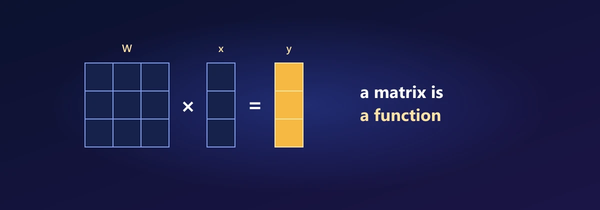
A matrix is a function: it takes in a vector and gives out a vector. And not just any function. It is a linear one, meaning it respects addition and scaling:
Linearity has a powerful consequence. Any vector can be built from the basis vectors e₁ = (1, 0, …), e₂ = (0, 1, …) and so on: x = x₁e₁ + x₂e₂ + …. So a linear function is completely determined by what it does to the basis vectors: f(x) = x₁f(e₁) + x₂f(e₂) + …. A matrix is nothing more than a list of those answers, written as columns. Column j of W is where W sends eⱼ.
W = torch.tensor([[2.0, -1.0], [1.0, 3.0]])
e1, e2 = torch.tensor([1.0, 0.0]), torch.tensor([0.0, 1.0])
print(W @ e1, W @ e2)                                # the columns of W
v = torch.tensor([4.0, 5.0])
print(W @ v, 4 * (W @ e1) + 5 * (W @ e2))            # the same: linearity at work

a, b, c = torch.randn(2), torch.randn(2), 3.7
print(torch.allclose(W @ (a + b), W @ a + W @ b), torch.allclose(W @ (c * a), c * (W @ a)))tensor([2., 1.]) tensor([-1., 3.]) tensor([ 3., 19.]) tensor([ 3., 19.]) True True
Geometrically, a 2 × 2 matrix moves every point in the plane: it can rotate, stretch, shear or reflect it, but straight lines stay straight and the origin stays put. A layer's weight matrix does the same in 784 dimensions, reshaping the space the data lives in.
Why does matrix multiplication work row by column?
Question 3: multiplying two matrices uses a strange rule, row of the first times column of the second. Who decided that?
Nobody chose it; it is forced. If B sends x to Bx and A then sends that to A(Bx), the combined function is also linear, so it is also a matrix, and we call that matrix AB. Its columns must be where the combined function sends the basis vectors: column j of AB is A(B eⱼ) = A times column j of B. Working that out entry by entry gives exactly the row-times-column rule:
The shape rule is just as natural: B takes vectors of size p to size n, and A takes size n to size m, so they can only be chained if B's output size equals A's input size. Matrix multiplication is function composition, and that's why (AB)x = A(Bx), and why AB is usually not equal to BA: rotating then stretching differs from stretching then rotating.
A = torch.randn(3, 4)
B = torch.randn(4, 2)
x = torch.randn(2)
print(torch.allclose((A @ B) @ x, A @ (B @ x), atol=1e-6))      # composition
entry = sum(A[1, k] * B[k, 0] for k in range(4))
print(torch.allclose(entry, (A @ B)[1, 0]))                       # row 1 dotted with column 0
S, R = torch.tensor([[2.0, 0.0], [0.0, 1.0]]), torch.tensor([[0.0, -1.0], [1.0, 0.0]])
print(S @ R, R @ S, sep="\n") # stretch-rotate != rotate-stretchTrue
True
tensor([[ 0., -2.],
[ 1., 0.]])
tensor([[ 0., -1.],
[ 2., 0.]])This explains Lesson 6's key fact before you get there: stacking two layers without an activation function between them gives W₂(W₁x) = (W₂W₁)x, which is one matrix, one layer. Depth only adds power if something non-linear sits between the layers.
Why does PyTorch compute x Wᵀ?
Question 4: the input batch has shape (64, 784) and the weight (128, 784). How do they multiply?
In maths we write y = W x with x as a column. In code, a batch stores one example per row, X of shape (64, 784). Writing each example as a row turns W x into x Wᵀ, since transposing a product reverses it: (W x)ᵀ = xᵀ Wᵀ. Stacking all 64 rows, the whole batch is one matrix product, which is exactly what nn.Linear computes:
X = torch.randn(64, 784)
Y = X @ layer.weight.T + layer.bias
print(Y.shape, torch.allclose(Y, layer(X), atol=1e-5))torch.Size([64, 128]) True
A whole batch through a whole layer is one matrix multiplication: 64 × 128 dot products of length 784, all independent of each other. That independence is why GPUs, which run thousands of small calculations in parallel, make deep learning fast.
Autograd: where gradients come from
Setting requires_grad=True tells PyTorch to record every operation on a tensor. Calling backward() on a result walks that record backwards with the chain rule and stores each gradient in .grad. Lesson 7 opens this up completely; here we need two practical facts:
w = torch.tensor(2.0, requires_grad=True)
loss = (3 * w - 1) ** 2          # d(loss)/dw = 2(3w - 1) * 3 = 30 at w = 2
loss.backward()
print(w.grad)                    # tensor(30.)

loss = (3 * w - 1) ** 2
loss.backward()
print(w.grad)                    # tensor(60.): gradients ADD UP across backward() calls
w.grad.zero_() # this is why the loop calls optimizer.zero_grad()tensor(30.) tensor(60.)
Gradients accumulate rather than overwrite (useful when one update is built from several backward passes), so the training loop must clear them before each step. And inside torch.no_grad(), nothing is recorded, which saves memory and time during evaluation.
Datasets and DataLoaders
A Dataset needs two methods: __len__ (how many examples) and __getitem__ (return example number i). Here is one for any pair of arrays:
from torch.utils.data import Dataset

class ArrayDataset(Dataset):
    def __init__(self, features, targets):
        self.features = torch.as_tensor(features, dtype=torch.float32)
        self.targets = torch.as_tensor(targets)

    def __len__(self):
        return len(self.targets)

    def __getitem__(self, i):
        return self.features[i], self.targets[i]

ds = ArrayDataset(torch.randn(1000, 5), torch.randint(0, 2, (1000,)))
loader = DataLoader(ds, batch_size=32, shuffle=True)
xb, yb = next(iter(loader))
print(len(ds), len(loader), xb.shape, yb.shape) # 1000 examples, 32 batches1000 32 torch.Size([32, 5]) torch.Size([32])
The DataLoader handles batching, shuffling, and (with num_workers) loading data in parallel while the GPU trains. Which raises a question about that shuffle=True.
Why shuffle, and why is a small batch good enough?
Question 5: each step uses only 64 of 60,000 images. Why does a gradient from such a small batch point the right way?
The loss over the full dataset is an average of per-example losses, so its gradient is the average of per-example gradients. A batch drawn at random is a random sample of those gradients, and the expected value of a random sample's average is the full average. In statistical language, the mini-batch gradient is an unbiased estimate of the full gradient. It is noisy, but Lesson 3 told us how noisy: the variance of an average of B independent samples is σ²/B, so its spread shrinks like 1/√B. Shuffling is what makes each batch a fair random sample; without it, a batch might contain only T-shirts, and its gradient would pull the model the wrong way.
torch.manual_seed(0)
X_all = torch.randn(10_000, 5)
y_all = X_all @ torch.tensor([1.0, -2.0, 0.5, 3.0, 0.0]) + 0.1 * torch.randn(10_000)
w = torch.zeros(5, requires_grad=True)

def gradient(idx):
    w.grad = None
    ((X_all[idx] @ w - y_all[idx]) ** 2).mean().backward()
    return w.grad.clone()

full = gradient(torch.arange(10_000))
batches = torch.stack([gradient(torch.randint(0, 10_000, (64,))) for _ in range(2000)])
print("full-data gradient:      ", full.numpy().round(2))
print("average of batch grads:  ", batches.mean(0).numpy().round(2))     # unbiased: matches
print("spread, batch of 64: ", batches.std(0).numpy().round(2))full-data gradient: [-2.07 3.97 -1.12 -6.06 0.12] average of batch grads: [-2.05 3.95 -1.14 -6.08 0.14] spread, batch of 64: [0.99 1.06 0.95 1.21 0.91]
Models as nn.Module
Any class that inherits from nn.Module and defines forward is a model. Layers assigned as attributes are registered automatically, so model.parameters() finds every weight for the optimizer, .to(device) moves them all, and state_dict() lists them for saving:
model.to("cpu")
for name, param in model.named_parameters():
    print(f"{name:20s} {tuple(param.shape)}")
print("total:", sum(p_.numel() for p_ in model.parameters()))

torch.save(model.state_dict(), "classifier.pt")          # save the weights
restored = Classifier()
restored.load_state_dict(torch.load("classifier.pt"))     # load them into a fresh model
print(f"restored model accuracy: {evaluate(restored, test_loader):.1%}")
model.to(device)layers.1.weight (128, 784) layers.1.bias (128,) layers.3.weight (10, 128) layers.3.bias (10,) total: 101770 restored model accuracy: 86.1%
model.train() and model.eval() switch the behaviour of layers that act differently while training, such as dropout and batch normalisation (Lesson 8). They don't stop gradients; torch.no_grad() does that.
Using the GPU
A tensor or model lives on one device. Everything in an operation must be on the same device, so the pattern is: move the model once with model.to(device), and move each batch inside the loop with .to(device). Forgetting one of them gives an error like "expected all tensors to be on the same device". On a Colab T4, the training script above runs several times faster than on the CPU, and the gap grows with bigger models and batches, since there are more independent dot products to run in parallel.
Summary
A PyTorch program is tensors, a Dataset and DataLoader, an nn.Module, a loss, an optimizer and a loop of forward, zero_grad, backward and step, with evaluation under eval() and no_grad(). Broadcasting lines shapes up from the right. A linear layer computes y = Wx + b, many dot products at once. A matrix is a linear function whose columns are the images of the basis vectors, and matrix multiplication is composition of such functions, which forces the row-times-column rule and the inner-dimension shape rule; batches are processed as Y = X Wᵀ + b. Gradients accumulate, so they must be zeroed each step, and a shuffled mini-batch gives an unbiased, noisy estimate of the full gradient whose spread shrinks like 1/√B.
Exercises
1. Change the hidden layer from 128 to 16 and then 512 neurons. How do accuracy and the parameter count change?
2. Find the 2 × 2 matrix that rotates every vector by 90° anticlockwise, using only the rule that its columns are where e₁ and e₂ go. Check it on a few vectors. What does applying it four times give, and why?
3. Without running code, predict the shape of (5, 1, 3) + (4, 1), or explain why it fails. Then check.
4. Show that (AB)ᵀ = BᵀAᵀ by comparing entry (i, j) on both sides, then verify with random tensors.
5. Set shuffle=False for the training loader and sort the training data by label. Train for one epoch. What happens to the accuracy, and why, in terms of Question 5?
6. Write a Dataset that loads the house-price data from Lesson 3 and train a two-layer network to predict price. Report the test error.
Comments