Deep Learning CourseLesson 4 of 16 22 min
Is My Model Any Good?
What you'll learn: how to tell whether a model is actually good. We'll train a fraud detector that scores 96% accuracy and then discover it is barely better than doing nothing. From there: train, validation and test sets, the confusion matrix, precision, recall, F1, ROC curves and AUC. The questions along the way lead to why we train on a loss but report accuracy, where the −log p in cross-entropy comes from (likelihood and the Bernoulli distribution), why F1 uses a harmonic mean, and how much to trust a test score (the binomial distribution).
Before you start: Lessons 1 to 3. You'll need probability distributions (Lesson 1 and Lesson 3) and the idea of a training loop.
A model with 96% accuracy
We generate a dataset of 10,000 card transactions, each described by 20 numeric features, where 5% are fraudulent. Then we train a small PyTorch network to spot fraud and measure its accuracy on transactions it hasn't seen:
import numpy as np
import torch
from torch import nn
from sklearn.datasets import make_classification
from sklearn.model_selection import train_test_split

X, y = make_classification(n_samples=10_000, n_features=20, n_informative=6,
                           weights=[0.95, 0.05], class_sep=0.8, random_state=0)
X_train, X_test, y_train, y_test = train_test_split(X, y, test_size=0.25, stratify=y, random_state=0)

mean, std = X_train.mean(axis=0), X_train.std(axis=0)              # standardise (Lesson 3)
Xtr = torch.tensor((X_train - mean) / std, dtype=torch.float32)
Xte = torch.tensor((X_test - mean) / std, dtype=torch.float32)
ytr = torch.tensor(y_train, dtype=torch.float32).unsqueeze(1)

torch.manual_seed(0)
model = nn.Sequential(nn.Linear(20, 32), nn.ReLU(), nn.Linear(32, 1))
optimizer = torch.optim.Adam(model.parameters(), lr=0.01)
loss_fn = nn.BCEWithLogitsLoss()
for step in range(300):
    loss = loss_fn(model(Xtr), ytr)
    optimizer.zero_grad()
    loss.backward()
    optimizer.step()

with torch.no_grad():
    scores = torch.sigmoid(model(Xte)).squeeze(1).numpy()    # probability of fraud
predictions = (scores >= 0.5).astype(int)
print(f"accuracy: {(predictions == y_test).mean():.1%}")accuracy: 96.1%
96% sounds excellent. Now compare it with a "model" that doesn't look at the data at all and declares every transaction legitimate:
always_legit = np.zeros_like(y_test)
print(f"accuracy of always saying 'legit': {(always_legit == y_test).mean():.1%}")accuracy of always saying 'legit': 94.5%
94.5%. Our network beats doing nothing by less than two percentage points. Nobody who saw the details would call it "96% accurate". When one class is rare, accuracy is dominated by the common class and hides almost everything that matters. We need better ways to look.
What just happened
Accuracy counts every mistake equally and every correct answer equally. With 95% legitimate transactions, the easy majority swamps the score. But the two kinds of mistakes have very different costs: missing a fraud loses money, while flagging a legitimate purchase annoys a customer. Evaluating a model means measuring each kind of success and failure separately, on data the model has never touched, and knowing how much to trust the numbers. We take those in turn.
Train, validation and test sets
A model is evaluated on data it didn't learn from, or the score measures memory, not skill. In practice we need three sets, not two. The training set fits the weights. The validation set is for every decision you make while developing: which architecture, which learning rate, which threshold, when to stop. The test set is touched once, at the very end, to report the final number.
Why a separate validation set? Because every decision tuned on the test set leaks a little information about it into the model. Try fifty settings and keep the one with the best test score, and that score is now optimistic: you've selected the luckiest of fifty. The test set must stay unseen to remain an honest estimate.
When data is scarce, k-fold cross-validation reuses it: split the training data into k parts, train k times, each time validating on a different part, and average the k scores. With stratify=y, as in our split above, each part keeps the same 5% fraud rate.
The confusion matrix
Split the predictions by what the model said and what was true. Every prediction falls into one of four boxes:
| Predicted fraud | Predicted legit | |
|---|---|---|
| Actually fraud | TP (true positive) | FN (false negative): missed fraud |
| Actually legit | FP (false positive): false alarm | TN (true negative) |
from sklearn.metrics import confusion_matrix

tn, fp, fn, tp = confusion_matrix(y_test, predictions).ravel()
print(f"caught fraud (TP): {tp}   missed fraud (FN): {fn}")
print(f"false alarms (FP): {fp} correct legit (TN): {tn}")caught fraud (TP): 54 missed fraud (FN): 83 false alarms (FP): 14 correct legit (TN): 2349
Now the problem is visible: of the 137 fraudulent transactions in the test set, the model misses 83, more than half. Accuracy is (TP + TN) / total, and the huge TN count carries it. Two numbers built from the matrix tell the real story.
Precision and recall
Precision answers "when the model raises an alarm, should I believe it?". Recall answers "how much fraud slips through?". A model that flags only the single most suspicious transaction can have perfect precision and terrible recall; a model that flags everything has perfect recall and terrible precision. The always-legit model has a recall of zero, which accuracy completely hid.
from sklearn.metrics import precision_score, recall_score, f1_score

print(f"precision: {precision_score(y_test, predictions):.2f}")
print(f"recall:    {recall_score(y_test, predictions):.2f}")
print(f"F1: {f1_score(y_test, predictions):.2f}")precision: 0.79 recall: 0.39 F1: 0.53
Why does F1 use a harmonic mean?
Question 1: F1 combines precision P and recall R into one number. Why not just average them?
The ordinary (arithmetic) average lets a high value hide a low one. The model that flags every transaction has R = 1 and P = 0.05, and their average is 0.525, which sounds respectable for a useless model. The harmonic mean averages the reciprocals, and the reciprocal of a small number is huge, so the result is dragged towards the smaller value: here F1 = 0.095. To score well on F1, a model must be good at both.
The harmonic mean is the natural average for rates. If you drive one kilometre at 30 km/h and another at 90 km/h, your average speed is not 60 but 45, the harmonic mean, because you spend more time on the slow kilometre. Substituting the definitions of P and R also shows F1 has a simple form in the confusion matrix:
P, R = 0.05, 1.0
print("arithmetic mean:", (P + R) / 2, "  harmonic mean (F1):", round(2 * P * R / (P + R), 3))
print("F1 from counts:", round(2 * tp / (2 * tp + fp + fn), 4), " sklearn:", round(f1_score(y_test, predictions), 4))arithmetic mean: 0.525 harmonic mean (F1): 0.095 F1 from counts: 0.5268 sklearn: 0.5268
Thresholds: trading precision for recall
The model outputs a probability of fraud; turning it into a yes or no needs a threshold, and 0.5 was an arbitrary choice. Lowering it flags more transactions: recall rises, precision falls. Which threshold is right is a business decision about the cost of each mistake, made on the validation set:
for threshold in [0.5, 0.3, 0.2, 0.1, 0.05]:
    pred = (scores >= threshold).astype(int)
    print(f"threshold {threshold:<5} precision {precision_score(y_test, pred):.2f}"
f" recall {recall_score(y_test, pred):.2f} F1 {f1_score(y_test, pred):.2f}")threshold 0.5 precision 0.79 recall 0.39 F1 0.53 threshold 0.3 precision 0.60 recall 0.49 F1 0.54 threshold 0.2 precision 0.49 recall 0.55 F1 0.52 threshold 0.1 precision 0.35 recall 0.68 F1 0.46 threshold 0.05 precision 0.25 recall 0.77 F1 0.38
ROC curves and AUC
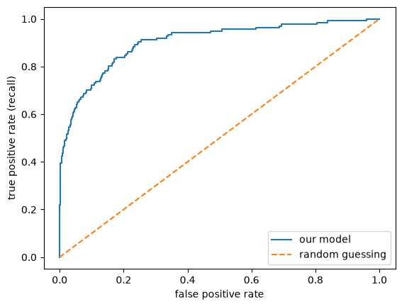
To evaluate the model across all thresholds at once, plot the true positive rate (recall) against the false positive rate, FP / (FP + TN), as the threshold sweeps from 1 down to 0. That is the ROC curve. A perfect model shoots straight up to the top-left corner; a model that guesses at random follows the diagonal. The area under the curve, AUC, summarises it in one number between 0.5 (random) and 1 (perfect):
from sklearn.metrics import roc_auc_score, roc_curve
import matplotlib.pyplot as plt

fpr, tpr, _ = roc_curve(y_test, scores)
print(f"AUC: {roc_auc_score(y_test, scores):.3f}")
plt.plot(fpr, tpr, label="our model")
plt.plot([0, 1], [0, 1], "--", label="random guessing")
plt.xlabel("false positive rate"); plt.ylabel("true positive rate (recall)")
plt.legend(); plt.show()AUC: 0.903
What does AUC actually measure?
Question 2: "area under a curve" is a strange thing to optimise. Does AUC have a plainer meaning?
It does, and it is one of the nicest facts in evaluation. AUC equals the probability that a randomly chosen fraudulent transaction gets a higher score than a randomly chosen legitimate one:
Why? Sweep the threshold down from the top. Each time it passes a positive example, the curve steps up; each time it passes a negative, the curve steps right. The area accumulated by each rightward step equals the fraction of positives already passed, which is the fraction of positives scored above that negative. Summing over all negatives gives the fraction of (positive, negative) pairs ranked correctly. So AUC measures ranking quality, independent of any threshold. We can check by brute force over every pair:
pos = scores[y_test == 1]
neg = scores[y_test == 0]
pairs_correct = (pos[:, None] > neg[None, :]).mean()       # compare every positive with every negative
print(f"fraction of pairs ranked correctly: {pairs_correct:.3f} sklearn AUC: {roc_auc_score(y_test, scores):.3f}")fraction of pairs ranked correctly: 0.903 sklearn AUC: 0.903
Why do we train on loss but report accuracy?
Question 3: if accuracy, recall and F1 are what we care about, why does the training loop minimise cross-entropy instead?
Because training needs gradients, and these metrics don't have useful ones. Accuracy counts predictions on the right side of a threshold. Nudge a weight slightly and either no prediction crosses the threshold, so accuracy doesn't change at all (derivative zero), or one prediction crosses and accuracy jumps (no derivative). As a function of the weights, accuracy is a staircase. Lesson 7 shows that gradient descent needs a function that is continuous and has a slope everywhere; a staircase gives no direction to move. The loss is a smooth stand-in: it rewards the model for putting more probability on the right answer, a little at a time.
w = torch.linspace(-3, 3, 7)
toy_x, toy_y = torch.tensor([1.0, -1.0, 2.0]), torch.tensor([1.0, 0.0, 1.0])
for wi in w:
    p_ = torch.sigmoid(wi * toy_x)
    acc = ((p_ >= 0.5).float() == toy_y).float().mean()
    bce = nn.functional.binary_cross_entropy(p_, toy_y)
print(f"weight {wi:+.1f}: accuracy {acc:.2f} loss {bce:.3f}")weight -3.0: accuracy 0.00 loss 4.033 weight -2.0: accuracy 0.00 loss 2.757 weight -1.0: accuracy 0.00 loss 1.584 weight +0.0: accuracy 0.67 loss 0.693 weight +1.0: accuracy 1.00 loss 0.251 weight +2.0: accuracy 1.00 loss 0.091 weight +3.0: accuracy 1.00 loss 0.033
As the weight changes, accuracy jumps between a few values, while the loss changes smoothly and keeps improving even after accuracy has stopped. But why that particular smooth function, −log of a probability?
Where does −log p come from?
Question 4: the binary cross-entropy loss is −[y log p + (1 − y) log(1 − p)]. Where does that formula come from?
Start with a fair question: how good is a model that predicts probabilities? A natural answer is to ask how probable the model thought the labels that actually happened were. That quantity is called the likelihood.
For a single yes/no outcome, the model's prediction p is a Bernoulli distribution: the simplest of all probability distributions, over two outcomes, with P(y = 1) = p and P(y = 0) = 1 − p. Both cases fit in one formula, because a number to the power 0 is 1:
Assuming the examples are independent, the probability of all n labels together is the product of the individual probabilities. Maximum likelihood estimation chooses the weights that make this product as large as possible:
But a product of thousands of numbers below 1 is astronomically small, too small for a computer to store, and products are awkward to differentiate. The logarithm fixes both: log turns products into sums, log(ab) = log a + log b, and because log is increasing, maximising the log of something maximises the thing itself. Finally, we prefer to minimise, so we flip the sign and average:
So the cross-entropy loss isn't an arbitrary formula. Minimising it is maximum likelihood: choosing the weights under which the observed labels were most probable. The same derivation with the categorical distribution, the multi-class version of the Bernoulli, gives the categorical cross-entropy used with softmax in Lesson 1. We can check both the underflow problem and the equivalence:
with torch.no_grad():
    p_train = torch.sigmoid(model(Xtr)).squeeze(1).double().numpy()
y_np = y_train

per_example = p_train ** y_np * (1 - p_train) ** (1 - y_np)       # Bernoulli probability of each label
print("product of all probabilities:", np.prod(per_example))     # about 1e-296: the edge of what a float can hold
print("with twice as much data:      ", np.prod(np.concatenate([per_example, per_example])))   # underflows to 0.0
log_likelihood = np.sum(np.log(per_example))
print("log-likelihood:", round(log_likelihood, 2))
print("-log-likelihood / n:", round(-log_likelihood / len(y_np), 5))
print("PyTorch BCE loss: ", round(loss_fn(model(Xtr), ytr).item(), 5)) # the same numberproduct of all probabilities: 1.858588505071179e-296 with twice as much data: 0.0 log-likelihood: -680.95 -log-likelihood / n: 0.09079 PyTorch BCE loss: 0.09079
How much should you trust a test score?
Question 5: model A scores 91% on 200 test examples and model B scores 90%. Is A really better?
Think of each test example as a coin flip that lands "correct" with probability equal to the model's true accuracy, a. The number of correct answers out of n is then a binomial random variable, the distribution of the number of successes in n independent yes/no trials:
The standard deviation follows from Lesson 3: each trial is a Bernoulli variable with variance a(1 − a), the variances of n independent trials add up to n·a(1 − a), and dividing the count by n to get a proportion divides the variance by n². With a = 0.9 and n = 200, the standard deviation is about 2.1 percentage points, and roughly 95% of measurements fall within two standard deviations, so a measured accuracy of anywhere from about 86% to 94% is unsurprising. A one-point difference between A and B on 200 examples is just noise. Simulation agrees:
rng = np.random.default_rng(0)
a, n_test = 0.90, 200
measured = rng.binomial(n_test, a, size=100_000) / n_test     # 100,000 imaginary test sets
print(f"theory: std {np.sqrt(a * (1 - a) / n_test):.4f}")
print(f"simulation: std {measured.std():.4f}, 95% of scores between "
      f"{np.percentile(measured, 2.5):.3f} and {np.percentile(measured, 97.5):.3f}")
print(f"how often a 90% model scores 91% or more by luck: {(measured >= 0.91).mean():.0%}")theory: std 0.0212 simulation: std 0.0212, 95% of scores between 0.855 and 0.940 how often a 90% model scores 91% or more by luck: 37%
A model with a true accuracy of 90% scores 91% or better on a 200-example test set more than a third of the time, purely by luck. Because the standard deviation shrinks only like 1/√n, halving the uncertainty takes four times as much test data. For our fraud detector the problem is worse: recall is measured on only 137 frauds, so its uncertainty is several points wide.
Summary
Evaluate on data the model hasn't seen: a training set for fitting, a validation set for every decision, and a test set used once. Accuracy misleads when classes are imbalanced. The confusion matrix separates true and false positives and negatives; precision is TP/(TP + FP), recall is TP/(TP + FN), and F1 is their harmonic mean, which punishes a weak side. The threshold trades precision for recall, the ROC curve shows every threshold at once, and AUC is the probability that a random positive outranks a random negative. We train on cross-entropy because metrics like accuracy are staircases with no useful gradient, and cross-entropy is the negative log-likelihood of a Bernoulli (or categorical) distribution. A measured accuracy has binomial noise with standard deviation √(a(1 − a)/n), so small differences on small test sets mean little.
Exercises
1. Compute precision, recall and F1 of the always-legit model by hand. Which of them is undefined, and why? What does sklearn report?
2. Show that if precision equals recall, then F1 equals both of them.
3. Retrain the fraud model with pos_weight in BCEWithLogitsLoss (try torch.tensor([10.0])) so that missed fraud costs ten times more. How do precision, recall and AUC change? Why does AUC change much less than the others?
4. Derive the loss for a single example when y = 1 and when y = 0, and sketch both as functions of p. Why does the loss go to infinity as p approaches the wrong extreme?
5. How many test examples would you need so that the standard deviation of a 90% accuracy is 0.5 percentage points? Check your answer by simulation.
6. Implement 5-fold cross-validation for the fraud model using sklearn's StratifiedKFold. How much does the AUC vary between folds, and does that match your expectation from Question 5?