Deep Learning Course · Lesson 3 of 16 · 25 min

Exploratory Data Analysis and the Statistics Behind It

Deepak Mishra, Senior Technology Lead at Incedo 10 November 2026

What you'll learn: how to inspect a dataset before training on it, find its problems (missing values, typos, outliers, mixed scales, text categories), and fix them with Pandas. The questions that come up along the way lead into the statistics every deep learning practitioner needs: mean and variance, why we divide by n − 1, probability distributions and the normal curve, correlation as an angle, and why scaling makes gradient descent faster.

Before you start: Lessons 0 to 2. Lesson 2's vectors, lengths and dot products come back here in a surprising place.

Five lines that find the problems

Lessons 1 and 2 used datasets someone else had cleaned. Real data is messy. To keep this lesson self-contained, we generate a house-price dataset (area, bedrooms, age, city and price in lakhs) and then damage it the way real data gets damaged: some values go missing, and one price gets an extra zero typed into it.

import numpy as np
import pandas as pd

rng = np.random.default_rng(42)
n = 200
area = rng.normal(1500, 400, n).round()      # square feet
bedrooms = rng.integers(1, 6, n)
age = rng.integers(0, 50, n)
city = rng.choice(["Delhi", "Mumbai", "Pune"], n, p=[0.5, 0.3, 0.2])
city_premium = pd.Series(city).map({"Delhi": 20, "Mumbai": 40, "Pune": 0}).to_numpy()
price = 50 + 0.08 * area + 5 * bedrooms - 0.6 * age + city_premium + rng.normal(0, 15, n)

df = pd.DataFrame({"area": area, "bedrooms": bedrooms, "age": age,
                   "city": city, "price": price.round(1)})
df.loc[rng.choice(n, 12, replace=False), "area"] = np.nan     # missing values
df.loc[rng.choice(n, 6, replace=False), "city"] = np.nan
df.loc[5, "price"] = df.loc[5, "price"] * 10                  # a data-entry error

Now pretend you've just been handed this file. These five lines are the first thing to run on any dataset:

print(df.head())                 # what does a row look like?
df.info()                        # column types, and how many values are present
print(df.describe())             # summary statistics of the numeric columns
print(df.isnull().sum())         # missing values per column
print(df["city"].value_counts()) # what categories are there?

     area  bedrooms  age   city  price
0  1622.0         5   48   Pune  158.6
1  1084.0         1   42   Pune  112.1
2  1800.0         1   41  Delhi  178.3
3     NaN         2   23   Pune  207.0
4   720.0         2   39  Delhi  144.2
<class 'pandas.DataFrame'>
RangeIndex: 200 entries, 0 to 199
Data columns (total 5 columns):
 #   Column    Non-Null Count  Dtype  
---  ------    --------------  -----  
 0   area      188 non-null    float64
 1   bedrooms  200 non-null    int64  
 2   age       200 non-null    int64  
 3   city      194 non-null    str    
 4   price     200 non-null    float64
dtypes: float64(2), int64(2), str(1)
memory usage: 7.9 KB
              area    bedrooms         age        price
count   188.000000  200.000000  200.000000   200.000000
mean   1482.218085    3.035000   25.645000   195.059000
std     349.323962    1.505025   14.132146    71.438488
min     647.000000    1.000000    0.000000    95.500000
25%    1234.750000    2.000000   14.000000   162.050000
50%    1473.000000    3.000000   26.000000   190.750000
75%    1696.000000    4.250000   38.000000   216.575000
max    2666.000000    5.000000   49.000000  1043.000000
area        12
bedrooms     0
age          0
city         6
price        0
dtype: int64
city
Delhi     92
Mumbai    63
Pune      39
Name: count, dtype: int64

Between them they reveal every problem we planted. info() and isnull() show 12 missing areas and 6 missing cities. describe() shows a maximum price of 1,043 when three quarters of houses cost under 217: a strong hint of an error. value_counts() shows city is text, which a network can't use. And the columns are on wildly different scales: area runs into thousands, bedrooms from 1 to 5. The rest of the lesson fixes each problem, and stops at each step to ask why.

What describe() is telling you

describe() reports, for each numeric column, the count, mean, standard deviation (std), minimum, quartiles (25%, 50%, 75%) and maximum. The mean is the average. The quartiles split the sorted values into four equal groups: a quarter of the houses are below the 25% value, half below the 50% value (the median), and three quarters below the 75% value. The standard deviation measures spread, and its definition prompts the first question.

Why square the deviations?

Question 1: to measure spread, why average the squared distances from the mean, rather than the distances themselves?

The plain deviations xᵢ − x̄ are useless on their own: they always sum to exactly zero, because the mean is the balance point. So we must get rid of the signs, and there are two obvious ways: absolute values |xᵢ − x̄|, or squares (xᵢ − x̄)². Squares win for three reasons.

First, squares are smooth. The absolute value has a corner at zero, which (as Lesson 7 shows) means no derivative there, while x² has a derivative everywhere, so every tool of calculus applies. Second, squares connect to geometry. Put all the deviations into one vector d = (x₁ − x̄, …, xₙ − x̄). Then Σ(xᵢ − x̄)² is d · d = ‖d‖², the squared length of that vector from Lesson 2. The standard deviation is simply the length of the deviation vector, rescaled: s = ‖d‖ / √(n − 1). Third, variances of independent quantities add, a fact we'll use in Question 5 and throughout the course.

prices = df["price"].to_numpy()
d = prices - prices.mean()                     # the deviation vector
print("deviations sum to:", round(d.sum(), 10))                       # 0
print("length-based std:", np.linalg.norm(d) / np.sqrt(len(d) - 1))
print("pandas std:      ", df["price"].std())                         # the same

deviations sum to: 0.0
length-based std: 71.4384875717051
pandas std:       71.4384875717051

Why divide by n − 1?

Question 2: the mean divides by n, but the variance divides by n − 1. Why the odd one out?

Our data is a sample from a much larger population (all the houses that could have been in the dataset). We want the population's variance σ², but we measure spread around the sample mean x̄ instead of the unknown population mean μ. The sample mean is, by construction, the point that minimises the sum of squared deviations for this particular sample, so the data always looks a little less spread out around x̄ than around the true μ. Dividing by n would underestimate σ² on average.

How much? The identity below follows by expanding the squares, writing xᵢ − μ = (xᵢ − x̄) + (x̄ − μ):

On average, the first sum on the right is nσ² (each term averages σ²), and the average of (x̄ − μ)² is σ²/n, the variance of a mean of n independent values (Question 5 explains why). So on average Σ(xᵢ − x̄)² equals nσ² − σ² = (n − 1)σ². Dividing by n − 1 corrects the bias exactly. This is called Bessel's correction. A simulation confirms it:

rng_sim = np.random.default_rng(0)
true_variance = 4.0                               # population: normal with sigma = 2
samples = rng_sim.normal(0, 2, size=(100_000, 5)) # 100,000 samples of size n = 5
print("divide by n:     ", samples.var(axis=1, ddof=0).mean())   # about 3.2 = (4/5) * 4
print("divide by n - 1: ", samples.var(axis=1, ddof=1).mean())   # about 4.0

divide by n:      3.2096590074453006
divide by n - 1:  4.0120737593066265

With samples of 5, dividing by n is too small by a factor of 4/5 on average, exactly as (n − 1)/n predicts. NumPy divides by n by default; pass ddof=1 to get n − 1, which is what Pandas uses.

Fixing missing values

With the statistics understood, the fixes are straightforward. For a numeric column, fill gaps with the median, which a single extreme value can't drag around (the mean can: one bad price moved the mean of price about 4 lakhs above its median). For a categorical column, fill with the most frequent value:

print("mean:", df["price"].mean().round(1), " median:", df["price"].median())

df["area"] = df["area"].fillna(df["area"].median())
df["city"] = df["city"].fillna(df["city"].mode()[0])
print("missing values left:", df.isnull().sum().sum())

mean: 195.1  median: 190.75
missing values left: 0

Imputation is a guess. In real projects it often helps to add a column such as area_was_missing, so the model can learn whether missingness itself carries information.

Looking at the shape of the data

Summary numbers hide the shape of the data. A histogram shows it, by counting how many values fall into each of a series of bins:

PythonCopy

import matplotlib.pyplot as plt

fig, axes = plt.subplots(1, 2, figsize=(11, 4))
df["area"].hist(bins=20, ax=axes[0]); axes[0].set_title("Area (sq ft)")
df["price"].hist(bins=20, ax=axes[1]); axes[1].set_title("Price (lakhs)")
plt.show()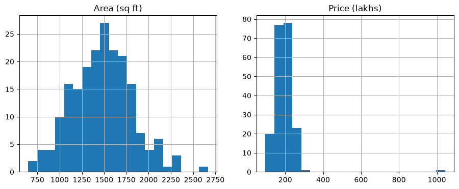

Output

The area histogram is a single symmetric hump. The price histogram is squashed against the left edge, with one lonely bar far out on the right: the typo. A histogram is an estimate of something more fundamental, which brings us to distributions.

What is a probability distribution for a measurement?

Question 3: Lesson 1 defined a probability distribution over 37 breeds. What is the equivalent for something like area, which can take any value?

For a list of separate outcomes, each outcome gets a probability. But area can be 1500, 1500.1, 1500.0001 square feet: infinitely many values, so each single value has probability zero. Instead, a continuous distribution is described by a probability density function (PDF) f(x), and probability is the area under its curve:

These are Lesson 1's two rules again, with the sum replaced by an integral (a sum of infinitely many infinitely thin slices). A histogram with its bar heights scaled so the total area is 1 is a rough picture of the density. The cumulative distribution function (CDF), F(x) = P(X ≤ x), adds up the area from the left, rising from 0 to 1; the median is where it crosses ½ and the quartiles where it crosses ¼ and ¾.

Why does the bell curve appear everywhere?

Question 4: the area histogram looks like a bell. Is there a reason so many measurements look like that?

The bell is the normal (Gaussian) distribution, with mean μ and standard deviation σ:

The exponent is the squared distance from the mean, measured in units of σ, so the density falls off rapidly as you move away from μ. The reason it is everywhere is the central limit theorem: when a quantity is the sum of many small, independent effects, its distribution approaches a normal distribution, whatever the distribution of the individual effects. Heights, measurement errors and exam scores are all sums of many small influences. Here we add up uniform random numbers (each one flat, nothing like a bell) and watch the bell appear:

PythonCopy

rng_clt = np.random.default_rng(1)
fig, axes = plt.subplots(1, 4, figsize=(16, 3))
for ax, k in zip(axes, [1, 2, 5, 30]):
    sums = rng_clt.uniform(0, 1, size=(100_000, k)).sum(axis=1)
    ax.hist(sums, bins=60, density=True)
    ax.set_title(f"sum of {k} uniform numbers")
plt.show()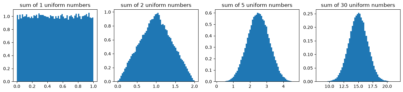

Output

How rare is "three standard deviations"?

Question 5: a common rule flags outliers more than 3 standard deviations from the mean. Why 3?

Measure each value by how many standard deviations it lies from the mean. This is the z-score, z = (x − μ)/σ. For a normal distribution, integrating the density gives the famous 68-95-99.7 rule: about 68% of values lie within 1σ of the mean, 95% within 2σ, and 99.7% within 3σ. So a value beyond 3σ happens only about 3 times in 1,000 by chance, and a value beyond 10σ essentially never. Let's check by simulation:

x = np.random.default_rng(2).normal(0, 1, 1_000_000)
for k in [1, 2, 3]:
    print(f"within {k} sigma: {np.mean(np.abs(x) < k):.4f}")

within 1 sigma: 0.6826
within 2 sigma: 0.9545
within 3 sigma: 0.9973

Two cautions. First, the rule assumes a roughly normal distribution; for skewed data, the IQR rule used by box plots is safer: flag anything more than 1.5 × IQR below the 25% quartile or above the 75% quartile, where IQR = Q3 − Q1. Second, an extreme value inflates the very standard deviation used to judge it. Both rules still catch our typo easily:

z = (df["price"] - df["price"].mean()) / df["price"].std()
print(df[z.abs() > 3])

q1, q3 = df["price"].quantile([0.25, 0.75])
iqr = q3 - q1
print(df[(df["price"] < q1 - 1.5 * iqr) | (df["price"] > q3 + 1.5 * iqr)])

    area  bedrooms  age  city   price
5  979.0         1   19  Pune  1043.0
    area  bedrooms  age  city   price
5  979.0         1   19  Pune  1043.0

We know row 5 is a typo, so we fix it. If you can't tell whether an outlier is an error, don't delete it blindly: check the row, ask someone who knows the data, or cap it at the fence.

df.loc[5, "price"] = df.loc[5, "price"] / 10
print("std of price after the fix:", round(df["price"].std(), 1))   # almost half what it was

std of price after the fix: 38.9

The answer to the last question is also why the variance of a mean is σ²/n, used in Question 2. Variances of independent quantities add: Var(X + Y) = Var(X) + Var(Y). Summing n independent values with variance σ² gives variance nσ², and dividing by n to get the mean divides the variance by n², leaving σ²/n. The spread of an average shrinks like 1/√n, which is also why averaging gradients over a mini-batch gives a steadier estimate (Lesson 7).

Which columns move together?

Next, find out which features are related to each other and to the price. Pearson's correlation coefficient r does this, and it always lies between −1 and +1:

print(df[["area", "bedrooms", "age", "price"]].corr().round(2))

          area  bedrooms   age  price
area      1.00      0.04  0.02   0.69
bedrooms  0.04      1.00 -0.17   0.30
age       0.02     -0.17  1.00  -0.31
price     0.69      0.30 -0.31   1.00

The matrix rediscovers what we built into the data: area is strongly positively correlated with price, age negatively, and bedrooms weakly positively. But look at the formula again, with Lesson 2 in mind.

Why is correlation always between −1 and 1?

Question 6: what is r, geometrically, and why can't it escape [−1, 1]?

Take the deviation vectors of the two columns, dₓ = (xᵢ − x̄) and d_y = (yᵢ − ȳ). The top of the formula is their dot product, and the bottom is the product of their lengths. So r is exactly the cosine similarity from Lesson 2:

Correlation is the cosine of an angle in a 200-dimensional space, one dimension per house. A cosine can't leave [−1, 1], and r = ±1 means the deviation vectors point in exactly the same or opposite directions, which happens only when y is a perfect straight-line function of x. Uncorrelated columns have perpendicular deviation vectors.

dx = df["area"] - df["area"].mean()
dy = df["price"] - df["price"].mean()
cosine = (dx @ dy) / (np.linalg.norm(dx) * np.linalg.norm(dy))
print(cosine, df["area"].corr(df["price"]))   # identical

0.6902023786277066 0.6902023786277066

Two cautions that follow from this picture. Correlation measures only straight-line relationships: a perfect U-shape can have r near 0. And correlation is not causation: ice-cream sales and drownings are correlated because both rise in summer.

Turning categories into numbers

A network can only multiply numbers, so city must become numeric. The tempting shortcut, Delhi = 0, Mumbai = 1, Pune = 2, quietly tells the model that Pune is "twice" Mumbai and that Mumbai lies between Delhi and Pune. In Lesson 2's language: it places the cities on a line, at unequal distances. One-hot encoding gives each category its own column instead:

df_encoded = pd.get_dummies(df, columns=["city"], dtype=int)
print(df_encoded.head())

delhi, mumbai, pune = np.eye(3)                 # the three one-hot vectors
print(np.linalg.norm(delhi - mumbai), np.linalg.norm(delhi - pune), np.linalg.norm(mumbai - pune))

     area  bedrooms  age  price  city_Delhi  city_Mumbai  city_Pune
0  1622.0         5   48  158.6           0            0          1
1  1084.0         1   42  112.1           0            0          1
2  1800.0         1   41  178.3           1            0          0
3  1473.0         2   23  207.0           0            0          1
4   720.0         2   39  144.2           1            0          0
1.4142135623730951 1.4142135623730951 1.4142135623730951

Every pair of one-hot vectors is the same distance apart, √2, and every pair is perpendicular. The encoding makes no claims about which cities are similar, leaving the model to learn that from the data.

Why does scaling make training faster?

Question 7: area is in the thousands, bedrooms in single digits. Why does that hurt training, and what does scaling fix?

Two standard rescalings put features on comparable ranges:

To see why it matters, fit a simple linear model, price ≈ w₁·area + w₂·bedrooms + b, by gradient descent. Lesson 7 shows that gradient descent is only stable when the learning rate is below 2/M, where M is the largest curvature of the loss. With unscaled features, the loss curves extremely steeply in the area direction (because area values are huge) and gently in the bedrooms direction. The learning rate has to be tiny to survive the steep direction, so progress in the gentle direction crawls. The loss surface is a long, narrow valley. Standardising makes the curvatures similar, the valley round, and a single learning rate works for every weight:

def fit(X, y, lr, steps=500):
    X = np.column_stack([X, np.ones(len(X))])      # add a column of ones for the bias
    w = np.zeros(X.shape[1])
    for _ in range(steps):
        w -= lr * 2 * X.T @ (X @ w - y) / len(y)   # gradient of the mean squared error
    return np.mean((X @ w - y) ** 2)

X_raw = df[["area", "bedrooms"]].to_numpy(dtype=float)
X_std = (X_raw - X_raw.mean(axis=0)) / X_raw.std(axis=0)
y = df["price"].to_numpy()

A = np.column_stack([X_raw, np.ones(len(X_raw))])
best = np.mean((A @ np.linalg.lstsq(A, y, rcond=None)[0] - y) ** 2)
print("best possible MSE:                     ", round(best, 1))
print("standardised, lr 0.1, 500 steps:       ", round(fit(X_std, y, lr=0.1), 1))
print("unscaled, lr 4e-7, 500 steps:          ", round(fit(X_raw, y, lr=4e-7), 1))
print("unscaled, lr 4e-7, 50,000 steps:       ", round(fit(X_raw, y, lr=4e-7, steps=50_000), 1))
print("unscaled, lr 4.5e-7, 500 steps:        ", fit(X_raw, y, lr=4.5e-7))

best possible MSE:                      671.1
standardised, lr 0.1, 500 steps:        671.1
unscaled, lr 4e-7, 500 steps:           1049.5
unscaled, lr 4e-7, 50,000 steps:        999.8
unscaled, lr 4.5e-7, 500 steps:         2.4184546603102287e+37

The standardised model reaches the best possible error in 500 steps. The unscaled model, at its largest stable learning rate, is still far away after 50,000 steps, and nudging the learning rate up by just 12% makes it explode. Any learning rate large enough to make progress in the gentle directions is too large for the steep area direction. The same applies to neural networks, which is why inputs are almost always standardised.

Split first, then scale

The model will be judged on data it has never seen, so set aside a test set before fitting anything, including the scaler. If you compute the mean and standard deviation from the full dataset, information about the test set leaks into training and the test score becomes optimistic. This mistake is called data leakage, and Lesson 4 is about measuring models honestly.

from sklearn.model_selection import train_test_split
from sklearn.preprocessing import StandardScaler

X = df_encoded.drop(columns="price")
y = df_encoded["price"]
X_train, X_test, y_train, y_test = train_test_split(X, y, test_size=0.2, random_state=42)

cols = ["area", "bedrooms", "age"]
scaler = StandardScaler()
X_train[cols] = scaler.fit_transform(X_train[cols])   # learn mean and std from train only
X_test[cols] = scaler.transform(X_test[cols])         # reuse them on test
print(X_train.shape, X_test.shape)

(160, 6) (40, 6)

Summary

Always start with head(), info(), describe(), isnull() and value_counts(). Variance averages squared deviations because squares are smooth and turn the deviations into a vector whose squared length is the total, and it divides by n − 1 because measuring around the sample mean underestimates spread by a factor of (n − 1)/n. Continuous measurements have probability densities, where area under the curve is probability; the normal distribution appears whenever many small independent effects add up (the central limit theorem), and its 68-95-99.7 rule justifies the 3σ outlier rule. Correlation is the cosine of the angle between deviation vectors. One-hot encoding keeps categories equidistant, standardisation makes gradient descent converge by evening out the curvature, and scalers are fitted on the training set only.

Exercises

1. Show that the deviations xᵢ − x̄ always sum to zero, for any data.

2. For the data 2, 4, 4, 4, 5, 5, 7, 9, compute the variance by hand with n and with n − 1, then check with NumPy.

3. Repeat the Bessel simulation with sample sizes 2, 10 and 100. How does the gap between the two estimates change, and does it match (n − 1)/n?

4. Generate y = x² for x evenly spaced from −1 to 1 and compute the correlation. Explain the result using the angle picture.

5. Draw 10,000 samples from an exponential distribution (rng.exponential), which is heavily skewed. What fraction lie more than 3 standard deviations above the mean? Compare with the 0.15% a normal distribution would give, and explain.

6. In the scaling experiment, find the largest learning rate for which the unscaled fit doesn't diverge. How does it compare with the standardised one? Relate the ratio to the spread of area and bedrooms.

Found this useful? Share it: LinkedIn X