Deep Learning CourseLesson 8 of 16 30 min
Training Well: Regularisation, Learning Rates and Tuning
What you'll learn: why a network can be perfect on its training data and poor on new data, and the toolkit for fixing it: weight decay, dropout, early stopping, data augmentation and batch normalisation, plus learning-rate schedules and hyperparameter search. The questions along the way lead into the bias-variance decomposition, Bayes' rule and why weight decay is a Gaussian prior, why L1 produces exact zeros, why decaying the learning rate helps, and why random search beats grid search.
Before you start: Lessons 1 to 7. You'll use expectations and variances (Lesson 3), likelihood (Lesson 4), the PyTorch loop (Lesson 5) and gradient descent (Lesson 7).
A network that memorises
Give a big network too little data and it will memorise it. Here a two-layer network with about 670,000 weights trains on only 1,000 Fashion-MNIST images, and we track its accuracy on those images and on 10,000 it never sees:
import numpy as np
import torch
from torch import nn
from torch.utils.data import DataLoader, Subset
from torchvision import datasets, transforms

tf = transforms.ToTensor()
full_train = datasets.FashionMNIST("data", train=True, download=True, transform=tf)
test_data = datasets.FashionMNIST("data", train=False, download=True, transform=tf)
small_train = Subset(full_train, range(1000))
train_loader = DataLoader(small_train, batch_size=50, shuffle=True)
test_loader = DataLoader(test_data, batch_size=1000)

def make_model(dropout=0.0):
    return nn.Sequential(nn.Flatten(),
                         nn.Linear(784, 512), nn.ReLU(), nn.Dropout(dropout),
                         nn.Linear(512, 512), nn.ReLU(), nn.Dropout(dropout),
                         nn.Linear(512, 10))

def accuracy(model, loader):
    model.eval()
    with torch.no_grad():
        return np.mean([(model(x).argmax(1) == y).float().mean().item() for x, y in loader])

def mean_loss(model, loader):
    model.eval()
    with torch.no_grad():
        return np.mean([nn.functional.cross_entropy(model(x), y).item() for x, y in loader])

def train(model, epochs=60, weight_decay=0.0, report_every=15):
    opt = torch.optim.AdamW(model.parameters(), lr=1e-3, weight_decay=weight_decay)
    for epoch in range(1, epochs + 1):
        model.train()
        for x, y in train_loader:
            loss = nn.functional.cross_entropy(model(x), y)
            opt.zero_grad(); loss.backward(); opt.step()
        if epoch % report_every == 0:
            print(f"epoch {epoch:2d}: train accuracy {accuracy(model, train_loader):.1%}"
                  f"   test accuracy {accuracy(model, test_loader):.1%}"
                  f"   test loss {mean_loss(model, test_loader):.2f}")
    return model

torch.manual_seed(0)
baseline = train(make_model())epoch 15: train accuracy 93.1% test accuracy 78.8% test loss 0.78 epoch 30: train accuracy 97.4% test accuracy 79.1% test loss 0.95 epoch 45: train accuracy 99.4% test accuracy 80.1% test loss 1.14 epoch 60: train accuracy 99.9% test accuracy 79.7% test loss 1.34
Training accuracy climbs to nearly 100%: the network has memorised its 1,000 images. Test accuracy stalls around 80%, and worse, the test loss keeps rising, from 0.78 to 1.34. The network is growing ever more confident in its answers, including the wrong ones (remember from Lesson 4 that cross-entropy punishes confident mistakes hard). This is overfitting, and the gap between training and test performance is its signature. Now the same network with two regularisers switched on, dropout and weight decay:
torch.manual_seed(0)
regularised = train(make_model(dropout=0.5), weight_decay=1.0)epoch 15: train accuracy 87.9% test accuracy 77.3% test loss 0.64 epoch 30: train accuracy 94.9% test accuracy 79.6% test loss 0.59 epoch 45: train accuracy 95.0% test accuracy 79.1% test loss 0.67 epoch 60: train accuracy 96.9% test accuracy 80.4% test loss 0.60
Now the training accuracy rises more slowly, the train-test gap is narrower, and the test loss stays flat instead of climbing. Notice what doesn't change much: test accuracy. On this problem, regularisation mainly stops the network from becoming overconfident; its predicted probabilities stay honest. On other problems, especially with augmentation and architectures suited to the data, it lifts accuracy too. Either way, the same data and the same network behave better. The rest of this lesson explains why these tricks work, and adds the others.
What just happened
A network with hundreds of thousands of weights has enough freedom to fit 1,000 examples exactly, including their accidents: the odd lighting in one photo, the unusual angle of another. Those accidents don't repeat in new data, so fitting them hurts. Regularisation means any technique that discourages a model from using all of its freedom unless the data really demands it. To choose techniques sensibly, it helps to split the error on new data into its parts.
Where does test error come from?
Question 1: why does a more flexible model sometimes do worse on new data?
Imagine training the same kind of model many times, each time on a fresh random training set, and predicting at one point x. Each training run gives a slightly different prediction f̂(x), so f̂(x) is a random variable. The true value is y = f(x) + ε, where ε is noise with variance σ². The expected squared error splits exactly into three parts:
The derivation is one idea: add and subtract E[f̂] inside the square, (y − f̂) = (y − f) + (f − E[f̂]) + (E[f̂] − f̂), expand, and use linearity of expectation. Every cross term has a factor with expected value zero (the noise averages to zero, and f̂ averages to E[f̂]), so only the three squares survive.
Bias is error from the model being systematically wrong, typically too simple to capture the pattern. Variance is error from the model being too sensitive to which training set it happened to get. Noise is the randomness no model can remove. Flexible models have low bias but high variance; regularisation trades a little bias for a big cut in variance. We can measure all three by simulation, fitting polynomials to noisy samples of a sine wave many times:
rng = np.random.default_rng(0)
f = lambda x: np.sin(np.pi * x)
x0, sigma = 0.5, 0.2                         # where we measure, and the noise level

for degree in [1, 3, 6]:
    preds = []
    for _ in range(2000):                    # 2,000 independent training sets of 15 points
        xs = rng.uniform(-1, 1, 15)
        ys = f(xs) + rng.normal(0, sigma, 15)
        coeffs = np.polyfit(xs, ys, degree)
        preds.append(np.polyval(coeffs, x0))
    preds = np.array(preds)
    y_new = f(x0) + rng.normal(0, sigma, 2000)
    bias2 = (f(x0) - preds.mean()) ** 2
    variance = preds.var()
    print(f"degree {degree}: bias^2 {bias2:.4f} + variance {variance:.4f} + noise {sigma**2:.4f}"
f" = {bias2 + variance + sigma**2:.4f} (measured error {np.mean((y_new - preds) ** 2):.4f})")degree 1: bias^2 0.2482 + variance 0.0340 + noise 0.0400 = 0.3222 (measured error 0.3248) degree 3: bias^2 0.0001 + variance 0.0131 + noise 0.0400 = 0.0532 (measured error 0.0525) degree 6: bias^2 0.0000 + variance 0.2176 + noise 0.0400 = 0.2576 (measured error 0.2551)
Plotting fits makes bias and variance visible. Each panel fits 20 polynomials of one degree, each to its own 15 noisy points from the same curve:
import matplotlib.pyplot as plt

grid = np.linspace(-1, 1, 200)
fig, axes = plt.subplots(1, 3, figsize=(15, 3.8), sharey=True)
for ax, degree in zip(axes, [1, 3, 6]):
    for _ in range(20):
        xs = rng.uniform(-1, 1, 15)
        ys = f(xs) + rng.normal(0, sigma, 15)
        ax.plot(grid, np.polyval(np.polyfit(xs, ys, degree), grid), color="tab:blue", alpha=0.25)
    ax.plot(grid, f(grid), color="black", linewidth=2, label="true curve")
    ax.set_title(f"degree {degree}"); ax.set_ylim(-2, 2)
axes[0].legend()
plt.show()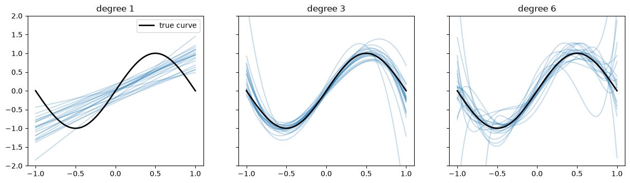
The straight line (degree 1) is dominated by bias; degree 6 has almost no bias but a large variance, because with only 15 points it bends to fit the noise; degree 3 balances them. And the three parts really do add up to the measured error.
Weight decay
Overfit models tend to have large weights, which is how they produce sharp, wiggly functions. L2 regularisation adds a penalty on the squared size of the weights to the loss:
The second line explains the name weight decay: before each normal step, every weight shrinks by a factor slightly below 1, and survives only if the data keeps pushing it back up. AdamW, which we used above, applies the decay in exactly this direct form. But why should small weights generalise better?
Why should small weights generalise better?
Question 2: is the L2 penalty just a heuristic, or does it follow from something?
It follows from Bayes' rule. Before seeing any data, we might believe that weights are probably small: a prior distribution p(w). After seeing the data D, the updated belief is the posterior:
Choosing the most probable weights under the posterior is called MAP (maximum a posteriori) estimation. As in Lesson 4, take the negative log to turn products into sums (and drop p(D), which doesn't depend on w):
The first term is the usual loss: Lesson 4 showed that minimising cross-entropy is maximising the likelihood. The second is a penalty that depends on the prior. If the prior says each weight is normally distributed around zero with standard deviation τ, its density is proportional to exp(−w²/(2τ²)), so −log p(w) = w²/(2τ²) + constant. That is exactly the L2 penalty, with λ = 1/τ². Weight decay is a Gaussian belief that weights are probably small; a strong penalty is a narrow prior.
Use a different prior and you get a different penalty. The Laplace distribution, with density proportional to exp(−|w|/b), has a sharp peak at zero and heavier tails. Its negative log is |w|/b: the L1 penalty, λ Σ |w|. Its sharp peak expresses the belief that many weights are exactly zero, and that is what L1 delivers.
w = np.linspace(-3, 3, 7)
gauss = np.exp(-w ** 2 / 2)            # Gaussian prior, tau = 1
laplace = np.exp(-np.abs(w))           # Laplace prior, b = 1
print("w:                  ", w)
print("-log Gaussian prior:", (-np.log(gauss)).round(2) + 0.0, " = w^2/2")
print("-log Laplace prior: ", (-np.log(laplace)).round(2) + 0.0, " = |w|")w: [-3. -2. -1. 0. 1. 2. 3.] -log Gaussian prior: [4.5 2. 0.5 0. 0.5 2. 4.5] = w^2/2 -log Laplace prior: [3. 2. 1. 0. 1. 2. 3.] = |w|
Why does L1 give exact zeros?
Question 3: L1 and L2 both shrink weights. Why does only L1 shrink some all the way to zero?
Look at the simplest case: one weight w, whose data loss alone would put it at a, so the loss is ½(w − a)². Add each penalty and find the best w. With L2, setting the derivative of ½(w − a)² + ½λw² to zero gives w = a/(1 + λ): every weight shrinks by the same factor and never reaches zero unless a was zero already.
With L1, ½(w − a)² + λ|w| has a corner at w = 0 (Lesson 7's |x|, which has no derivative there). Away from zero the slope is (w − a) ± λ, and at zero the best you can say is that any slope between −λ and +λ fits (a subgradient). So w = 0 is optimal whenever |a| ≤ λ: the penalty's pull at zero is strong enough to hold any weakly supported weight there exactly. Otherwise w moves λ towards zero. This is soft-thresholding:
grid = np.linspace(-3, 3, 600_001)                 # brute-force minimisation on a fine grid
lam = 1.0
for a in [2.5, 0.8, -0.3, -1.7]:
    l1 = grid[np.argmin(0.5 * (grid - a) ** 2 + lam * np.abs(grid))] + 0.0
    l2 = grid[np.argmin(0.5 * (grid - a) ** 2 + 0.5 * lam * grid ** 2)]
    print(f"a = {a:+.1f}:  L1 best {l1:+.3f} (formula {np.sign(a) * max(abs(a) - lam, 0) + 0.0:+.3f})"
f" L2 best {l2:+.3f} (formula {a / (1 + lam):+.3f})")a = +2.5: L1 best +1.500 (formula +1.500) L2 best +1.250 (formula +1.250) a = +0.8: L1 best +0.000 (formula +0.000) L2 best +0.400 (formula +0.400) a = -0.3: L1 best +0.000 (formula +0.000) L2 best -0.150 (formula -0.150) a = -1.7: L1 best -0.700 (formula -0.700) L2 best -0.850 (formula -0.850)
L1 therefore produces sparse models, which doubles as automatic feature selection. In deep networks L2 (weight decay) is far more common; L1 is useful when you want to know which inputs matter.
Dropout
Dropout zeroes each neuron's output at random during training, with probability 1 − p, so every mini-batch trains a different thinned-out network. A neuron can no longer rely on particular partners being present, so it must learn features that are useful on their own. A network with n droppable neurons is in effect an ensemble of 2ⁿ sub-networks sharing weights, and averaging many models is a classic way to reduce variance.
Question 4: if neurons vanish during training but not at test time, won't the next layer see bigger inputs at test time?
It would, so frameworks use inverted dropout: during training the surviving activations are divided by p. Each neuron is multiplied by a mask m that is 1 with probability p and 0 otherwise, a Bernoulli variable from Lesson 4, whose expected value is p. So the expected output is unchanged:
drop = nn.Dropout(0.3)              # PyTorch takes the DROP probability, 1 - p
a = torch.ones(10_000)
drop.train(); out = drop(a)
print("zeroed:", (out == 0).float().mean().item(), " surviving value:", out.max().item(),
      " mean:", out.mean().item())
drop.eval(); print("at test time:", drop(a).mean().item())zeroed: 0.30309998989105225 surviving value: 1.4285714626312256 mean: 0.9955715537071228 at test time: 1.0
Early stopping
Track the validation loss as training goes on. At first it falls with the training loss; at some point it bottoms out and rises while the training loss keeps falling. From there on the network is memorising. Early stopping keeps the weights from the best validation epoch and stops after a set number of epochs without improvement (the patience). It's cheap and almost always worth using, and it acts much like weight decay: weights don't get the time to grow large.
import copy

def train_early_stopping(model, val_loader, patience=5, max_epochs=100):
    opt = torch.optim.AdamW(model.parameters(), lr=1e-3)
    best_acc, best_state, bad_epochs = 0.0, None, 0
    for epoch in range(max_epochs):
        model.train()
        for x, y in train_loader:
            loss = nn.functional.cross_entropy(model(x), y)
            opt.zero_grad(); loss.backward(); opt.step()
        val_acc = accuracy(model, val_loader)
        if val_acc > best_acc:
            best_acc, best_state, bad_epochs = val_acc, copy.deepcopy(model.state_dict()), 0
        else:
            bad_epochs += 1
            if bad_epochs == patience:
                break
    model.load_state_dict(best_state)
    return epoch + 1, best_acc

val_loader = DataLoader(Subset(full_train, range(50_000, 52_000)), batch_size=1000)   # held-out images
torch.manual_seed(0)
epochs_run, best = train_early_stopping(make_model(dropout=0.5), val_loader)
print(f"stopped after {epochs_run} epochs, best validation accuracy {best:.1%}")stopped after 24 epochs, best validation accuracy 81.5%
Data augmentation
The most reliable cure for overfitting is more data, and often you can manufacture it. A shirt flipped left to right, shifted a few pixels or slightly rotated is still a shirt, so each training image can appear in many variations. The network learns that these changes don't alter the answer, which is exactly the generalisation we want. In torchvision, augmentations are transforms applied each time an image is loaded, so every epoch sees fresh variations:
augment = transforms.Compose([
    transforms.RandomHorizontalFlip(),
    transforms.RandomAffine(degrees=10, translate=(0.1, 0.1)),
    transforms.ToTensor(),
])
augmented_train = datasets.FashionMNIST("data", train=True, download=True, transform=augment)
img1, _ = augmented_train[0]
img2, _ = augmented_train[0]
print("same image, two loads, identical?", torch.equal(img1, img2)) # almost always Falsesame image, two loads, identical? False
Batch normalisation
Batch normalisation standardises each feature over the current mini-batch (Lesson 3's z-score) and then lets the network rescale and shift it with two learned parameters, γ and β:
Its main benefit is faster, more stable training: each layer's inputs keep a steady distribution, which tolerates higher learning rates and worse initialisation. It also regularises slightly, because each example's normalisation depends on which other examples share its batch, adding noise. At test time a single example has no batch, so the layer uses running averages of μ and σ² collected during training; model.eval() switches that on, which is one reason forgetting eval() gives strange test results.
Learning-rate schedules
Question 5: Lesson 7 showed the learning rate must be small enough to be stable. Why do modern recipes also change it during training?
With mini-batches, every gradient is noisy (Lesson 5). Near a minimum, the true gradient is small but the noise isn't, so with a fixed learning rate the weights keep getting kicked around the minimum, in a band whose size grows with η. A large η early on makes fast progress; a small η late on lets the weights settle into the bottom. Decaying the learning rate gets both. Here is noisy gradient descent on L(w) = w², with the same number of steps:
def noisy_descent(lr_schedule, steps=2000, seed=0):
    rng = np.random.default_rng(seed)
    w = 5.0
    for t in range(steps):
        grad = 2 * w + rng.normal(0, 2.0)        # true gradient plus mini-batch noise
        w -= lr_schedule(t) * grad
    return abs(w)

T = 2000
schedules = {
    "constant 0.1": lambda t: 0.1,
    "constant 0.001": lambda t: 0.001,
    "cosine 0.1 -> 0": lambda t: 0.5 * 0.1 * (1 + np.cos(np.pi * t / T)),
}
for name, schedule in schedules.items():
    final = np.mean([noisy_descent(schedule, seed=s) for s in range(200)])
print(f"{name:16s}: average distance from the minimum after {T} steps: {final:.4f}")constant 0.1 : average distance from the minimum after 2000 steps: 0.2627 constant 0.001 : average distance from the minimum after 2000 steps: 0.0891 cosine 0.1 -> 0 : average distance from the minimum after 2000 steps: 0.0410
The large constant rate gets close quickly but keeps bouncing; the small one is steady but hasn't arrived; the cosine schedule, which starts large and glides down to zero, ends far closer than either. The cosine schedule, η_t = ½ η_max (1 + cos(πt/T)), is a common default, often preceded by a short warmup in which the rate rises from near zero, because the curvature at the start of training (random weights) can be large. In PyTorch: torch.optim.lr_scheduler.CosineAnnealingLR, stepped once per epoch or batch.
Hyperparameter search
Learning rate, weight decay, dropout, batch size and width are hyperparameters: settings chosen by you, not learned. You tune them by training several models and comparing them on the validation set (never the test set, as Lesson 4 explained).
Question 6: is it better to try a regular grid of values, or random values?
Random, usually. Two reasons. First, a simple probability argument: if each random trial independently has a 5% chance of landing in the best 5% of settings, the chance that none of n trials does is 0.95ⁿ, so the chance that at least one does is 1 − 0.95ⁿ. Sixty random trials give 1 − 0.95⁶⁰ ≈ 95%, whatever the number of hyperparameters. Second, usually only one or two hyperparameters matter much. A 3 × 3 grid over two of them tries only 3 distinct values of the important one, while 9 random trials try 9. Learning rates and weight decays are best sampled on a log scale (uniformly in the exponent), because their effect depends on their order of magnitude:
rng = np.random.default_rng(0)
print("chance at least one of n random trials is in the top 5%:",
      {n: round(1 - 0.95 ** n, 3) for n in [10, 30, 60]})

hits = np.mean([(rng.uniform(size=60) > 0.95).any() for _ in range(100_000)])
print("simulated with 60 trials:", round(hits, 3))

def important_only(lr, wd):          # pretend only the learning rate matters
    return -(np.log10(lr) + 2.5) ** 2

grid = [(lr, wd) for lr in [1e-4, 1e-3, 1e-2] for wd in [1e-4, 1e-3, 1e-2]]
random_trials = [(10 ** rng.uniform(-4, -2), 10 ** rng.uniform(-4, -2)) for _ in range(9)]
print("distinct learning rates tried: grid", len({lr for lr, _ in grid}),
      " random", len({lr for lr, _ in random_trials}))
print("best score: grid", round(max(important_only(*t) for t in grid), 3),
" random", round(max(important_only(*t) for t in random_trials), 3))chance at least one of n random trials is in the top 5%: {10: 0.401, 30: 0.785, 60: 0.954}
simulated with 60 trials: 0.953
distinct learning rates tried: grid 3 random 9
best score: grid -0.25 random -0.021Summary
Overfitting shows as a gap between training and validation performance. Expected test error splits into bias² + variance + noise, and regularisation trades a little bias for less variance. L2 weight decay shrinks weights each step and is MAP estimation with a Gaussian prior; L1 corresponds to a Laplace prior and, through soft-thresholding, sets weakly supported weights exactly to zero. Dropout zeroes random neurons and rescales the rest by 1/p, keeping the expected activation unchanged. Early stopping keeps the best validation epoch, augmentation manufactures data, and batch normalisation stabilises training. Decaying the learning rate lets noisy SGD settle into a minimum, and random search, on a log scale for rates, finds good hyperparameters more reliably than a grid.
Exercises
1. Re-run the overfitting experiment with 5,000 training images instead of 1,000, without regularisation. How does the train-test gap change? Relate it to the variance term.
2. Fill in the bias-variance derivation: expand the square of the three-term sum and show why each cross term has expectation zero.
3. Show that for linear regression, minimising the squared error plus ½λ‖w‖² gives w = (XᵀX + λI)⁻¹Xᵀy, and verify it against a gradient-descent solution.
4. Train the small-data network with weight decay values 0, 0.01, 0.1 and 1. Plot test accuracy against weight decay. Where is the best value, and what happens beyond it?
5. Prove that the variance of a·m/p (with m Bernoulli with probability p) is a²(1 − p)/p. What does that say about very aggressive dropout?
6. Add a warmup of 100 steps to the cosine schedule in the noisy descent experiment, starting the noise much larger in the first steps. Does warmup help?