Deep Learning CourseLesson 9 of 16 32 min
Convolutional Neural Networks for Computer Vision
What you'll learn: how convolutional neural networks (CNNs) see. We start by beating Lesson 5's clothing classifier with a CNN a third of its size, then look inside at the filters it learned. From there: the convolution operation, padding, stride and pooling, and the architectures behind modern vision. The questions along the way show that a convolution is just a matrix with shared weights, prove why shifting an image shifts the output, derive the output-size formula, measure what each neuron can see, and explain how skip connections keep gradients alive in very deep networks.
Before you start: Lessons 1 to 8, especially matrices as functions (Lesson 5) and vanishing gradients (Lesson 7).
A smaller network that sees better
Lesson 5's dense network flattened each 28 × 28 image into 784 numbers and reached about 86% on Fashion-MNIST with about 100,000 weights. This CNN keeps the image as a grid and slides small learned filters over it:
import numpy as np
import torch
from torch import nn
import torch.nn.functional as F
from torch.utils.data import DataLoader
from torchvision import datasets, transforms

tf = transforms.ToTensor()
train_data = datasets.FashionMNIST("data", train=True, download=True, transform=tf)
test_data = datasets.FashionMNIST("data", train=False, download=True, transform=tf)
train_loader = DataLoader(train_data, batch_size=64, shuffle=True)
test_loader = DataLoader(test_data, batch_size=1000)

torch.manual_seed(0)
cnn = nn.Sequential(
    nn.Conv2d(1, 32, kernel_size=3), nn.ReLU(), nn.MaxPool2d(2),    # 28x28 -> 26x26 -> 13x13
    nn.Conv2d(32, 64, kernel_size=3), nn.ReLU(), nn.MaxPool2d(2),   # 13x13 -> 11x11 -> 5x5
    nn.Flatten(),
    nn.Linear(64 * 5 * 5, 10),
)
optimizer = torch.optim.Adam(cnn.parameters(), lr=1e-3)

for epoch in range(2):
    cnn.train()
    for images, labels in train_loader:
        loss = F.cross_entropy(cnn(images), labels)
        optimizer.zero_grad(); loss.backward(); optimizer.step()
    cnn.eval()
    with torch.no_grad():
        acc = np.mean([(cnn(x).argmax(1) == y).float().mean().item() for x, y in test_loader])
    print(f"epoch {epoch + 1}: test accuracy {acc:.1%}")
print("parameters:", sum(p_.numel() for p_ in cnn.parameters()))epoch 1: test accuracy 86.3% epoch 2: test accuracy 87.8% parameters: 34826
About 88% after two epochs, with 34,826 parameters: better accuracy than Lesson 5's three epochs, from a third of the weights. The architecture itself carries knowledge about images, and that's what this lesson is about.
What just happened
The dense network had to learn, separately for every pixel position, what patterns matter there. A shirt collar at the top-left and the same collar one pixel lower are, to it, unrelated inputs. The CNN builds in two facts about images. Local connectivity: patterns such as edges, corners and textures are made of nearby pixels, so each neuron looks only at a small patch. Weight sharing: a pattern that matters in one place matters everywhere, so the same small filter is used at every position. We can look at the 32 filters the first layer learned, each just 3 × 3 weights, and at what one of them detects in an image:
import matplotlib.pyplot as plt

filters = cnn[0].weight.detach()                  # (32, 1, 3, 3)
image, label = test_data[0]
maps = F.relu(cnn[0](image.unsqueeze(0)))[0].detach()   # 32 feature maps, 26 x 26

fig, axes = plt.subplots(2, 8, figsize=(14, 4))
for i in range(8):
    axes[0, i].imshow(filters[i, 0].numpy(), cmap="gray"); axes[0, i].set_title(f"filter {i}")
    axes[1, i].imshow(maps[i].numpy(), cmap="gray")
for ax in axes.flat: ax.axis("off")
plt.show()
print("one filter's weights:\n", filters[0, 0].numpy().round(2))one filter's weights: [[-0.08 0.2 -0.28] [-0.32 -0.05 0.19] [-0.03 0.35 0.04]]
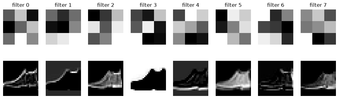
Each feature map lights up where its filter's pattern appears: some respond to vertical edges, some to horizontal edges, some to bright or dark regions. Nobody designed these filters; backpropagation found them. Let's see exactly what a filter computes.
The convolution operation
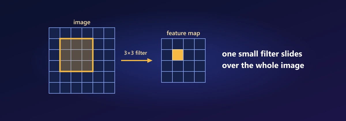
Place a small filter (kernel) K over the top-left patch of the image, multiply each filter weight by the pixel beneath it, and add everything up, plus a bias. That's one output number. Slide the filter one step and repeat, row by row. The grid of outputs is a feature map:
Each output is a dot product (Lesson 2) between the filter and one patch, so it measures how much that patch looks like the filter. A worked example: a 5 × 5 image, bright (10) on the left and dark (0) on the right, and a vertical-edge filter:
def conv2d(image, kernel, stride=1, padding=0):
    if padding:
        image = np.pad(image, padding)
    f = kernel.shape[0]
    out = (image.shape[0] - f) // stride + 1
    result = np.zeros((out, out))
    for i in range(out):
        for j in range(out):
            patch = image[i * stride:i * stride + f, j * stride:j * stride + f]
            result[i, j] = np.sum(patch * kernel)
    return result

I = np.array([[10, 10, 10, 0, 0]] * 5, dtype=float)
K = np.array([[1, 0, -1]] * 3, dtype=float)
print(conv2d(I, K))

# PyTorch's conv2d computes exactly the same thing
torch_out = F.conv2d(torch.tensor(I)[None, None], torch.tensor(K)[None, None])[0, 0]
print(np.allclose(conv2d(I, K), torch_out.numpy()))[[ 0. 30. 30.] [ 0. 30. 30.] [ 0. 30. 30.]] True
(Strictly, this is cross-correlation; textbook convolution flips the kernel first. Since the kernel weights are learned, the flip makes no difference, and every framework computes it this way.)
Is a convolution a new kind of layer?
Question 1: a convolution looks very different from nn.Linear. Is it really something new?
No. A convolution is linear: convolving the sum of two images gives the sum of their convolutions, and scaling an image scales the output. Lesson 5 showed that every linear function is a matrix. So a convolution is a matrix multiplication, just with a very special matrix. In one dimension, a 3-weight filter (k₀, k₁, k₂) sliding over a 6-number signal is this 4 × 6 matrix:
k = np.array([1.0, 0.0, -1.0])
signal = np.array([3.0, 5.0, 2.0, 8.0, 1.0, 4.0])
M = np.zeros((4, 6))
for row in range(4):
    M[row, row:row + 3] = k                       # the filter, shifted along each row
print(M @ signal)
print(np.array([signal[i:i + 3] @ k for i in range(4)])) # sliding the filter: identical[ 1. -3. 1. 4.] [ 1. -3. 1. 4.]
A CNN is a dense network whose weight matrices are forced to be mostly zero, with the remaining entries copied along the diagonals. That constraint is why it needs so few parameters, and why it generalises so well on images: it can't waste parameters learning a separate collar detector for every position.
Why does shifting the image shift the output?
Question 2: if a shirt moves two pixels to the right, what happens to the feature maps?
They move two pixels to the right as well, and nothing else changes. This property is called translation equivariance. The proof is a change of variables. Let I'(x, y) = I(x − a, y − b) be the image shifted by (a, b). Then
The output of the shifted image is the shifted output. The same filter weights are used at every position, so a pattern produces the same response wherever it appears. (At the borders the equality breaks down, because some patches fall off the edge; in the middle it is exact.)
img = torch.zeros(1, 1, 20, 20)
img[0, 0, 5:9, 5:9] = 1.0                                   # a small square
shifted = torch.roll(img, shifts=(3, 2), dims=(2, 3))      # move it down 3, right 2
conv = cnn[0]
with torch.no_grad():
    out, out_shifted = conv(img), conv(shifted)
print(torch.allclose(torch.roll(out, shifts=(3, 2), dims=(2, 3))[..., 4:14, 4:14],
out_shifted[..., 4:14, 4:14], atol=1e-6)) # same response, movedTrue
Padding, stride and the output size
Without padding each convolution shrinks the image, because the filter can't be centred on border pixels. Padding adds a border of p zeros on every side. Stride s is how far the filter moves each step; stride 2 roughly halves the width and height.
Question 3: how big is the output for any image size n, filter size f, padding p and stride s?
Count the positions where the filter fits. After padding, the image is n + 2p wide. The filter's left edge can start at 0, s, 2s, … and the last start must leave room for the filter, so it can't exceed n + 2p − f. The number of starts in 0, s, 2s, … up to that limit is:
x = torch.zeros(1, 1, 28, 28)
for pad, stride in [(0, 1), (1, 1), (1, 2)]:
    out = nn.Conv2d(1, 1, kernel_size=3, padding=pad, stride=stride)(x)
    print(f"padding {pad}, stride {stride}: {tuple(out.shape[2:])}"
f" formula: {(28 + 2 * pad - 3) // stride + 1}")padding 0, stride 1: (26, 26) formula: 26 padding 1, stride 1: (28, 28) formula: 28 padding 1, stride 2: (14, 14) formula: 14
Channels and parameters
A colour image has 3 channels, so each filter in the first layer is actually 3 × 3 × 3: it looks at the same patch in all channels and still outputs one number per position. A layer with C_out filters produces C_out feature maps, which become the channels of the next layer's input:
Unlike a dense layer, the count doesn't depend on the image size at all: the same filters work on a 28 × 28 image or a 4,000 × 3,000 photo.
Pooling
Max pooling shrinks each feature map by keeping only the largest value in each 2 × 2 window (with stride 2), halving the width and height. It keeps the strongest response ("there's an edge around here") and discards its exact position, so a small shift of the image often doesn't change the pooled output at all. Pooling has no parameters and works on each channel separately:
x = torch.tensor([[1, 3, 2, 1],
                  [4, 6, 5, 2],
                  [3, 1, 1, 0],
                  [2, 2, 4, 3]], dtype=torch.float32)[None, None]
print(F.max_pool2d(x, 2)[0, 0])                      # [[6, 5], [3, 4]]
shifted = torch.roll(x, shifts=1, dims=3)            # shift right by one pixel
print(F.max_pool2d(shifted, 2)[0, 0]) # partly unchangedtensor([[6., 5.],
[3., 4.]])
tensor([[4., 6.],
[3., 4.]])How much of the image does a neuron see?
Question 4: a first-layer neuron sees a 3 × 3 patch. How much of the image does a neuron deep in the network depend on?
Its receptive field grows with every layer. A second-layer neuron sees a 3 × 3 patch of first-layer outputs, each of which saw 3 × 3 pixels, overlapping by all but one pixel, so together they cover 5 × 5. Pooling multiplies the growth, because each step of a later layer jumps two pixels in the input. Instead of working it out by hand, we can measure it with autograd: backpropagate from a single output neuron to the input image, and see which pixels receive a non-zero gradient. Those are exactly the pixels it depends on. One subtlety: max pooling passes the gradient only to the winning pixel of each window, and ReLU blocks it wherever the input was negative, so for one particular image they hide part of the field. To measure everything a neuron could depend on, we use a stand-in with the same layer sizes, average pooling and no ReLU:
stand_in = nn.Sequential(nn.Conv2d(1, 1, 3), nn.AvgPool2d(2), nn.Conv2d(1, 1, 3), nn.AvgPool2d(2))
for layer in stand_in:
    if isinstance(layer, nn.Conv2d):
        nn.init.constant_(layer.weight, 1.0)          # all-positive weights: no accidental zeros

def receptive_field(layers, size=28):
    x = torch.randn(1, 1, size, size, requires_grad=True)
    out = layers(x)
    centre = (out.shape[2] // 2, out.shape[3] // 2)
    out[0, 0, centre[0], centre[1]].backward()       # gradient of one neuron
    return (x.grad[0, 0].abs().sum(dim=1) > 0).sum().item()   # rows it depends on

for n_layers, name in [(1, "conv1"), (2, "conv1 + pool"), (3, "conv2"), (4, "conv2 + pool")]:
print(f"after {name:13s} {receptive_field(stand_in[:n_layers])} pixels wide")after conv1 3 pixels wide after conv1 + pool 4 pixels wide after conv2 8 pixels wide after conv2 + pool 10 pixels wide
This growth is how CNNs build a hierarchy. Early layers, with tiny receptive fields, can only detect edges and colour changes. Middle layers combine those into textures, corners and simple shapes. Deep layers, which see most of the image, respond to object parts and whole objects.
Very deep networks and skip connections
Question 5: if depth helps, why not stack 100 convolutional layers?
Lesson 7 answered half of it: the backward pass multiplies by one layer's derivative after another, and over many layers the gradient vanishes or explodes. Until 2015, networks beyond about 20 layers trained worse than shallower ones. ResNet fixed it with a skip connection: each block learns a correction F(x) and adds it to its own input:
By the chain rule, the gradient through the block is the block's own derivative plus the identity. Even if ∂F/∂x is small, the I passes the gradient straight through, so it reaches the early layers undiminished. Let's compare the gradient reaching the input of 50 stacked layers, with and without skips:
def input_gradient(skip, depth=50, width=64):
    torch.manual_seed(0)
    blocks = [nn.Sequential(nn.Linear(width, width), nn.Tanh()) for _ in range(depth)]
    for block in blocks:
        nn.init.normal_(block[0].weight, std=0.5 / width ** 0.5)
    x = torch.randn(1, width, requires_grad=True)
    h_ = x
    for block in blocks:
        h_ = block(h_) + h_ if skip else block(h_)
    h_.sum().backward()
    return x.grad.norm().item()

print("50 layers, no skips:  ", input_gradient(skip=False))
print("50 layers, with skips:", input_gradient(skip=True))50 layers, no skips: 2.792244322382038e-15 50 layers, with skips: 52.955322265625
Without skips the gradient that reaches the input is around 10⁻¹⁵, effectively zero; with them it arrives at a healthy size. Skip connections made networks of 50, 152 and even 1,000 layers trainable, and they now appear in nearly every deep architecture, including the transformers of Lesson 12.
Landmark architectures
LeNet-5 (Yann LeCun, 1998) read handwritten digits on bank cheques, with the conv-pool-dense pattern we used. AlexNet (2012) won the ImageNet competition by a huge margin with a deeper CNN, ReLU, dropout and GPUs, and started the deep learning boom. VGG (2014) showed that stacks of small 3 × 3 filters work well: two of them see a 5 × 5 region with fewer parameters than one 5 × 5 filter. ResNet (2015) added skip connections. Later designs such as EfficientNet tuned depth, width and resolution together, and vision transformers (2020) apply the attention mechanism of Lesson 12 to patches of an image.
Transfer learning, revisited
Lesson 1 fine-tuned a pretrained ResNet-18. Now you know what was inside: early layers with general edge and texture filters, deep layers with object-part detectors, and skip connections throughout. Freezing the backbone and training a new head works because those features transfer to almost any image task. With more data, unfreezing the whole network and training it with a small learning rate (fine-tuning) usually does better still.
from torchvision import models

resnet = models.resnet18(weights=models.ResNet18_Weights.DEFAULT)
first_filters = resnet.conv1.weight.detach()          # 64 filters, each 3 x 7 x 7
print(first_filters.shape)
print("total parameters:", sum(p_.numel() for p_ in resnet.parameters()))torch.Size([64, 3, 7, 7]) total parameters: 11689512
Beyond classification
The same building blocks do much more than label images. Object detection (YOLO, Faster R-CNN) predicts a box and a class for every object in a picture. Semantic segmentation (U-Net) labels every pixel, which is widely used for tumours in medical scans. Face recognition maps faces to vectors compared by distance (Lesson 2). And the diffusion models of Lesson 15 use a U-Net to turn noise into images.
Summary
A CNN slides small learned filters over an image, S(i, j) = Σ I(i+m, j+n)·K(m, n) + b, each output a dot product measuring how much a patch looks like the filter. A convolution is a matrix multiplication with a sparse, weight-shared matrix, which is why it needs so few parameters, (f·f·C_in + 1)·C_out per layer regardless of image size. It is translation equivariant: shifting the input shifts the output. The output size is ⌊(n + 2p − f)/s⌋ + 1, pooling shrinks maps and adds tolerance to small shifts, and receptive fields grow with depth, giving a hierarchy from edges to objects. Skip connections, y = F(x) + x, add an identity to every block's derivative so gradients survive very deep networks.
Exercises
1. Write the 3 × 3 filter that detects horizontal edges and apply it to a test image with your conv2d. Then try a 3 × 3 blur filter (all weights 1/9).
2. Build the matrix for a 1D convolution of a 5-weight filter over a 10-number signal with stride 2. What shape is it, and how many of its entries are zero?
3. Compute by hand the output shape after each layer of a network with: conv 5×5 (padding 2), max pool 2, conv 3×3 (no padding), max pool 2, starting from 32 × 32. Check with PyTorch.
4. Work out the receptive field of our CNN's final conv layer by hand, then compare with the autograd measurement.
5. Replace the CNN's MaxPool2d layers with Conv2d layers using stride 2. How do accuracy and the parameter count change?
6. In the skip-connection experiment, try depths 5, 20 and 100, and plot the input gradient norm with and without skips on a log scale.
Comments