Deep Learning CourseLesson 16 of 16 17 min
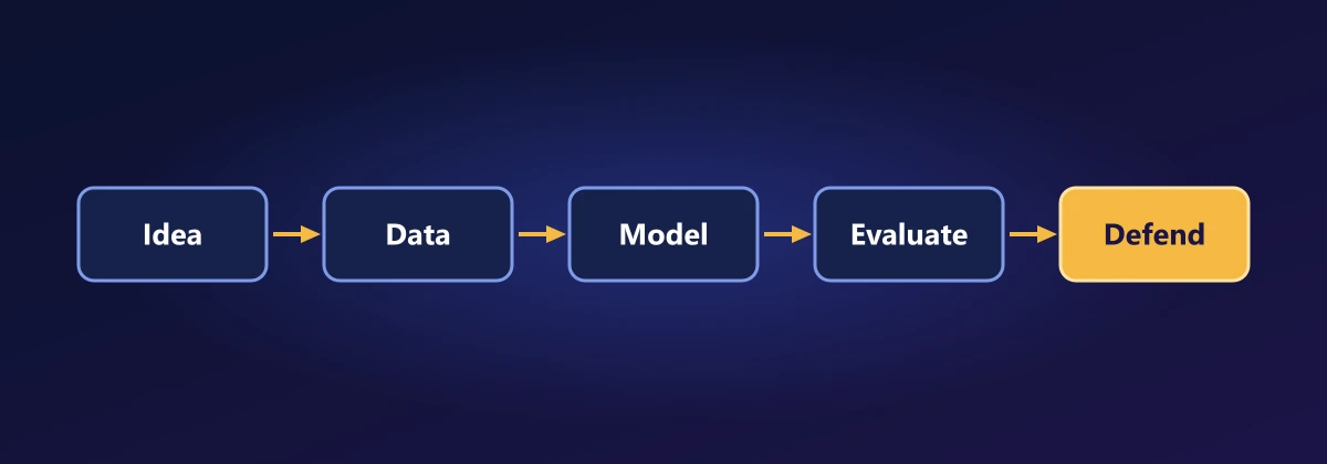
Capstone Project
What you'll do: build a complete deep learning project of your own choosing, from a question and raw data to a model you can defend with evidence. This lesson gives you the project options, a plan that maps each stage to the lesson that taught it, a reusable PyTorch template, and an evaluation checklist. One last question leads to the bootstrap: how to tell whether an improvement is real or luck.
Before you start: the whole course. Expect the project to take several sessions; the lesson itself is short, because the work is yours.
Start from a working skeleton
Every project in this course has had the same shape: data, a model, a training loop with validation, and an honest test. Here is that shape as one reusable template, run end to end on stand-in data so you can see it work before you swap in your own:
import copy
import numpy as np
import torch
from torch import nn
from torch.utils.data import DataLoader, TensorDataset, random_split

def set_seed(seed=0):
    np.random.seed(seed); torch.manual_seed(seed)

def make_loaders(dataset, batch_size=64, val_fraction=0.15, test_fraction=0.15, seed=0):
    n = len(dataset)
    n_val, n_test = int(n * val_fraction), int(n * test_fraction)
    train, val, test = random_split(dataset, [n - n_val - n_test, n_val, n_test],
                                    generator=torch.Generator().manual_seed(seed))
    return (DataLoader(train, batch_size, shuffle=True),
            DataLoader(val, batch_size), DataLoader(test, batch_size))

def evaluate(model, loader, device):
    model.eval()
    preds, targets = [], []
    with torch.no_grad():
        for x, y in loader:
            preds.append(model(x.to(device)).argmax(1).cpu()); targets.append(y)
    return torch.cat(preds), torch.cat(targets)

def train(model, train_loader, val_loader, epochs=50, lr=1e-3, weight_decay=1e-2, patience=5):
    device = "cuda" if torch.cuda.is_available() else "cpu"
    model.to(device)
    optimizer = torch.optim.AdamW(model.parameters(), lr=lr, weight_decay=weight_decay)
    scheduler = torch.optim.lr_scheduler.CosineAnnealingLR(optimizer, T_max=epochs)
    best_acc, best_state, waited = -1.0, None, 0
    for epoch in range(epochs):
        model.train()
        for x, y in train_loader:
            loss = nn.functional.cross_entropy(model(x.to(device)), y.to(device))
            optimizer.zero_grad(); loss.backward(); optimizer.step()
        scheduler.step()
        preds, targets = evaluate(model, val_loader, device)
        val_acc = (preds == targets).float().mean().item()
        if val_acc > best_acc:
            best_acc, best_state, waited = val_acc, copy.deepcopy(model.state_dict()), 0
        else:
            waited += 1
            if waited == patience:                      # early stopping (Lesson 8)
                break
    model.load_state_dict(best_state)
    return model, best_acc, epoch + 1

# Stand-in data: replace with your own Dataset
set_seed(0)
X = torch.randn(3000, 20)
y = (X[:, :3].sum(dim=1) + 0.5 * torch.randn(3000) > 0).long()
train_loader, val_loader, test_loader = make_loaders(TensorDataset(X, y))

model = nn.Sequential(nn.Linear(20, 64), nn.ReLU(), nn.Dropout(0.2), nn.Linear(64, 2))
model, val_acc, epochs_run = train(model, train_loader, val_loader)
preds, targets = evaluate(model, test_loader, "cpu")
test_correct = (preds == targets).float()
print(f"stopped after {epochs_run} epochs; validation accuracy {val_acc:.1%}; test accuracy {test_correct.mean():.1%}")stopped after 15 epochs; validation accuracy 89.3%; test accuracy 89.8%
Splits with a fixed seed, AdamW with weight decay, a cosine learning-rate schedule, early stopping on the validation set, and a test set touched once at the end: the template bakes in the habits of Lessons 4, 5 and 8. Your project replaces the stand-in data and the model.
Choose a project
Pick something you care about, with data you can actually get. Each option below draws on a different part of the course; any of them, done carefully, is a strong project.
1. Image classifier for a real problem (Lessons 1 and 9): plant diseases from leaf photos, defects in product images, or types of litter. Start from a pretrained ResNet, fine-tune, and study the mistakes.
2. Text classifier or assistant over your own documents (Lessons 2, 11 and 13): route support emails, detect spam in a community forum, or build a RAG assistant that answers questions about a set of documents and cites them.
3. Forecaster for a time series (Lessons 3 and 10): electricity demand, air quality, or footfall. Beat the naive "tomorrow equals today" baseline and show by how much, with an error bar.
4. Tabular predictor (Lessons 3, 4 and 8): churn, loan default or house prices, with careful exploratory analysis, honest metrics for imbalanced classes and a comparison against a simple model.
5. Generative model (Lessons 14 and 15): a diffusion model or VAE for a small image dataset of your own, with an evaluation of sample quality and diversity.
Plan the work
Work through the stages in order, and keep a short log of every decision and result; it becomes your report.
1. Frame the question (Lesson 4). What exactly is predicted or generated, for whom, and what would count as good enough? Choose the metric before you train anything: accuracy, recall at a given precision, mean squared error, or a human rating.
2. Get to know the data (Lesson 3). Inspect it, clean it, and look for leakage: any column or duplicate that wouldn't be available at prediction time. Fix the train, validation and test split now and don't move it.
3. Build a baseline (Lessons 4 and 10). The simplest thing that could work: the majority class, a naive forecast, logistic regression, or a pretrained model used as-is. Every later model must beat it.
4. Get to a first deep model fast (Lessons 1, 2 and 5). Use pretrained models where you can, and get something end to end before polishing anything.
5. Improve on the validation set (Lessons 6 to 13). Change one thing at a time: architecture, regularisation, learning rate, augmentation, more data. Random search over hyperparameters beats guessing.
6. Analyse errors. Look at the examples the model gets wrong, especially the confident ones. Mistakes usually reveal problems with the data or the labels, not just the model.
7. Test once, and report honestly. Evaluate the final model on the untouched test set, with an error bar, and describe where it fails.
Is my improvement real?
Question 1: your new model scores 1.5 points higher than the old one on the test set. Is it actually better, or did it get lucky with which examples happened to be in the test set?
Lesson 4 answered this with a formula, the binomial standard deviation √(a(1 − a)/n). The bootstrap answers it for any metric, with no formula at all. The idea: the test set is a sample from the world, so resampling it imitates drawing new test sets. Draw n examples from your n test examples with replacement (some appear twice, some not at all), recompute the metric, and repeat thousands of times. The spread of those recomputed values estimates how much the metric would vary from test set to test set:
def bootstrap_interval(correct, n_boot=10_000, seed=0):
    rng = np.random.default_rng(seed)
    correct = np.asarray(correct, dtype=float)
    means = [correct[rng.integers(0, len(correct), len(correct))].mean() for _ in range(n_boot)]
    return np.percentile(means, [2.5, 97.5])

low, high = bootstrap_interval(test_correct.numpy())
a, n = test_correct.mean().item(), len(test_correct)
print(f"test accuracy {a:.1%}, bootstrap 95% interval {low:.1%} to {high:.1%}")
print(f"binomial formula, +/- 2 standard deviations: {a - 2 * np.sqrt(a * (1 - a) / n):.1%} to {a + 2 * np.sqrt(a * (1 - a) / n):.1%}")test accuracy 89.8%, bootstrap 95% interval 86.9% to 92.4% binomial formula, +/- 2 standard deviations: 86.9% to 92.6%
For accuracy the bootstrap and Lesson 4's formula agree, which is a good check. But the bootstrap works just as well for F1, AUC, the median error, or any metric you can compute, where no simple formula exists.
Question 2: both models were scored on the same test examples. Can we use that?
Yes, and it makes the comparison much sharper. Many examples are easy (both models get them right) or impossible (both get them wrong); they say nothing about which model is better. Bootstrap the difference on each resample, keeping the pairing, and the shared easy and hard examples cancel out. If the interval for the difference lies entirely above zero, the improvement is unlikely to be luck:
rng = np.random.default_rng(1)
n_test = 500
model_a = (rng.random(n_test) < 0.85).astype(float)                  # 1 = correct on that example
flip = rng.random(n_test)
model_b = model_a.copy()
model_b[(model_a == 0) & (flip < 0.25)] = 1                          # B fixes some of A's mistakes
model_b[(model_a == 1) & (flip < 0.005)] = 0                         # and breaks a few of A's successes
print(f"accuracy A {model_a.mean():.1%}   B {model_b.mean():.1%}")

def paired_bootstrap(a, b, n_boot=10_000, seed=0):
    rng = np.random.default_rng(seed)
    diffs = []
    for _ in range(n_boot):
        idx = rng.integers(0, len(a), len(a))                        # the SAME examples for both
        diffs.append(b[idx].mean() - a[idx].mean())
    return np.percentile(diffs, [2.5, 97.5])

low, high = paired_bootstrap(model_a, model_b)
print(f"paired 95% interval for B - A: {low:+.1%} to {high:+.1%}")
unpaired_halfwidth = 2 * np.sqrt(model_a.var() / n_test + model_b.var() / n_test)
print(f"if the two scores were treated as independent: +/- {unpaired_halfwidth:.1%}")accuracy A 86.8% B 89.2% paired 95% interval for B - A: +1.0% to +4.0% if the two scores were treated as independent: +/- 4.1%
The paired interval is far narrower than the one you'd get by treating the two accuracies as independent, so a real improvement that the unpaired view would dismiss as noise becomes clearly visible. Use the paired bootstrap whenever you compare models on the same test set.
Evaluation checklist
Before you call the project finished, check each of these:
1. The test set was used once, at the end, and nothing (scaling, feature selection, early stopping, hyperparameters) was fitted on it.
2. There is a simple baseline, and the final model beats it by more than the error bar.
3. The metric matches the question, with precision, recall or per-class results for imbalanced problems.
4. Results come with uncertainty: a bootstrap interval, or results over several random seeds.
5. You've looked at the errors and can describe what kinds of input the model fails on.
6. You've checked for leakage: duplicates across splits, future information in time series, or labels hiding in the features.
7. Someone else could rerun your notebook from top to bottom and get the same numbers.
Report
Write the project up as a notebook plus a one- or two-page report: the question and why it matters; the data and how you cleaned and split it; the baseline; what you tried, in order, with validation results; the final test result with its interval; an analysis of errors; and what you'd do next with more time or data. Clear, honest reporting of a modest result is worth more than an impressive number nobody can trust.
Summary
A good project frames its question and metric first, studies and splits its data before modelling, beats a simple baseline, improves one change at a time on a validation set, analyses its errors, and reports a single test result with honest uncertainty. The bootstrap estimates that uncertainty for any metric by resampling the test set with replacement, and the paired bootstrap compares two models on the same examples far more precisely than treating their scores as independent.
Exercises
1. Run the template on the Lesson 3 house-price data (as a regression: change the loss to mean squared error and the evaluation to RMSE).
2. Show that the probability a particular example is left out of one bootstrap resample is (1 − 1/n)ⁿ, and that this approaches 1/e ≈ 37% as n grows. Check by simulation.
3. Bootstrap the AUC of Lesson 4's fraud model. How wide is the interval, and is it wider or narrower than for accuracy? Why?
4. Train the same model with five different random seeds. Is the spread across seeds larger or smaller than the bootstrap interval from one run? What does each measure?
5. Choose your project, write its question and metric in one sentence each, and build the baseline.
Comments