Deep Learning CourseLesson 15 of 16 25 min
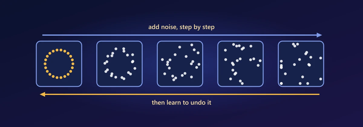
Diffusion Models and Generative AI
What you'll learn: how diffusion models create images from pure noise, by building one yourself, and how all of today's generative AI fits together. We start with Stable Diffusion, then train a small diffusion model from scratch that learns to generate a two-dimensional shape. Then we step back to generative AI as a whole: generative versus discriminative models, the main families of models, synthetic data, and the questions machines as creators raise. The questions along the way lead to Bayes' rule, why sums of Gaussian noise stay Gaussian (which lets diffusion jump to any step at once), why predicting the noise is enough, and how the reverse process removes it.
Before you start: Lessons 1 to 14, especially the normal distribution and variances of sums (Lesson 3), likelihood (Lesson 4), CNNs and U-Nets (Lesson 9), attention (Lesson 12) and VAEs (Lesson 14).
Generate an image from a sentence
On a Colab GPU, the diffusers library runs Stable Diffusion in a few lines. Type a description and get an image no one has drawn before:
import torch
from diffusers import StableDiffusionPipeline

pipe = StableDiffusionPipeline.from_pretrained(
    "stable-diffusion-v1-5/stable-diffusion-v1-5", torch_dtype=torch.float16
).to("cuda")

image = pipe("a watercolour painting of a lighthouse at sunrise",
             num_inference_steps=30, guidance_scale=7.5).images[0]
image.save("lighthouse.png")
The image starts as random static and is cleaned up in 30 steps, each guided by your sentence. That process, turning noise into data a little at a time, is what this lesson builds from scratch, on a problem small enough to train on a laptop in a couple of minutes.
Build a diffusion model
Our "images" are points in two dimensions, and the data is the two-moons shape: two interleaving half-circles. A diffusion model will learn to turn random points into points on the moons. The whole thing, data, noise schedule, a small denoising network, training and sampling, fits in one cell:
import numpy as np
import torch
from torch import nn
from sklearn.datasets import make_moons
import matplotlib.pyplot as plt

data = torch.tensor(make_moons(5000, noise=0.05, random_state=0)[0], dtype=torch.float32)
data = (data - data.mean(0)) / data.std(0)                 # standardise (Lesson 3)

T = 100                                                    # number of noise steps
betas = torch.linspace(1e-4, 0.1, T)                       # how much noise each step adds
alphas = 1 - betas
alpha_bar = torch.cumprod(alphas, dim=0)                   # alpha_1 * alpha_2 * ... * alpha_t

class Denoiser(nn.Module):                                 # predicts the noise in x_t
    def __init__(self):
        super().__init__()
        self.net = nn.Sequential(nn.Linear(3, 128), nn.SiLU(), nn.Linear(128, 128), nn.SiLU(),
                                 nn.Linear(128, 128), nn.SiLU(), nn.Linear(128, 2))
    def forward(self, x, t):
        return self.net(torch.cat([x, (t.float() / T).unsqueeze(1)], dim=1))

torch.manual_seed(0)
model = Denoiser()
optimizer = torch.optim.Adam(model.parameters(), lr=1e-3)
for step in range(5000):                                   # training
    x0 = data[torch.randint(0, len(data), (256,))]
    t = torch.randint(0, T, (256,))
    noise = torch.randn_like(x0)
    ab = alpha_bar[t].unsqueeze(1)
    x_t = ab.sqrt() * x0 + (1 - ab).sqrt() * noise         # jump straight to step t
    loss = ((model(x_t, t) - noise) ** 2).mean()           # learn to predict the noise
    optimizer.zero_grad(); loss.backward(); optimizer.step()

with torch.no_grad():                                      # sampling: start from pure noise
    x = torch.randn(1000, 2)
    start = x.clone()
    for t in reversed(range(T)):
        predicted = model(x, torch.full((1000,), t))
        x = (x - betas[t] / (1 - alpha_bar[t]).sqrt() * predicted) / alphas[t].sqrt()
        if t > 0:
            x = x + betas[t].sqrt() * torch.randn_like(x)

def fraction_near_data(points, radius=0.1):
    return (torch.cdist(points, data).min(dim=1).values < radius).float().mean().item()
print(f"points within 0.1 of the real data: noise {fraction_near_data(start):.0%}, generated {fraction_near_data(x):.0%}")

fig, axes = plt.subplots(1, 3, figsize=(13, 4))
for ax, pts, title in zip(axes, [data[:1000], start, x], ["real data", "starting noise", "generated"]):
    ax.scatter(pts[:, 0], pts[:, 1], s=3); ax.set_title(title); ax.set_aspect("equal")
plt.show()points within 0.1 of the real data: noise 38%, generated 90%
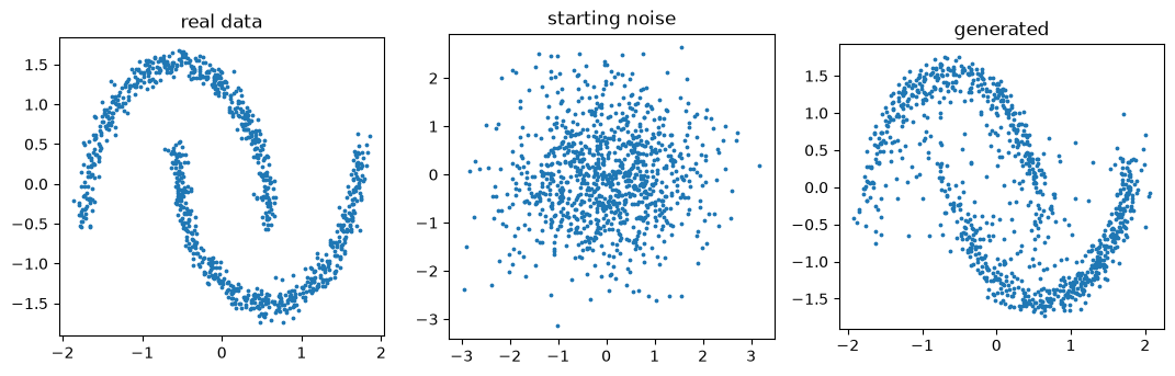
A cloud of random points has become two clear moons, apart from a few stray points: about 90% of the generated points lie within 0.1 of the real data, against under 40% for the starting noise. Stable Diffusion is this same algorithm, with images instead of points, a large U-Net instead of a small MLP, and text guiding the denoiser.
What just happened
The model learned a single skill: given a noisy point and how noisy it is (the step t), predict the noise that was added. Training made noisy versions of real points at random noise levels and graded the predictions. Generation then started from pure noise and repeatedly subtracted a little of the predicted noise, walking every point back towards the data. Two parts of the code deserve questions: the line that jumps straight to step t, and the update in the sampling loop.
The forward process
The forward process destroys data gradually. Each step shrinks the point slightly and adds a little Gaussian noise, with βₜ setting how much:
The shrinking factor √(1 − βₜ) is chosen so that the variance stays at 1: if xₜ₋₁ has variance 1, then xₜ has variance (1 − βₜ) + βₜ = 1. After enough steps nothing of the original remains, and xₜ is pure standard normal noise. That's the point: sampling then starts from a distribution we know exactly. But the training loop never runs these steps one by one.
Why can we jump straight to step t?
Question 1: the training code computes x_t = √ᾱₜ · x₀ + √(1 − ᾱₜ) · ε in one line. How can a single draw of noise replace t separate steps?
Two facts from Lesson 3 do it. Multiplying a normal variable by a constant c multiplies its standard deviation by c. And the sum of independent normal variables is normal, with the variances adding. Start from x₀ and take two steps:
The pattern continues by induction: after t steps the signal has been scaled by √(α₁α₂…αₜ) = √ᾱₜ, and all the noise added along the way combines into a single Gaussian with variance 1 − ᾱₜ. So x_t = √ᾱₜ x₀ + √(1 − ᾱₜ) ε exactly, in distribution. Training can pick any t at random and get its noisy example in one line. Let's confirm that 60 individual steps and the one-line jump give the same distribution:
torch.manual_seed(1)
x0_fixed = torch.tensor([1.5, -0.5])
t_check = 60
step_by_step = x0_fixed.repeat(100_000, 1)
for s in range(t_check):
    step_by_step = alphas[s].sqrt() * step_by_step + betas[s].sqrt() * torch.randn_like(step_by_step)
one_jump = alpha_bar[t_check - 1].sqrt() * x0_fixed + (1 - alpha_bar[t_check - 1]).sqrt() * torch.randn(100_000, 2)
print("step by step: mean", step_by_step.mean(0).numpy().round(3), " std", step_by_step.std(0).numpy().round(3))
print("one jump: mean", one_jump.mean(0).numpy().round(3), " std", one_jump.std(0).numpy().round(3))step by step: mean [ 0.607 -0.202] std [0.919 0.914] one jump: mean [ 0.603 -0.197] std [0.918 0.917]
Why predict the noise?
Question 2: we want to recover clean data. Why train the network to predict the noise instead?
Because knowing one gives you the other. Rearrange the jump formula: if you know x_t and the noise ε that was added, the clean point is fully determined:
Predicting ε is a well-scaled regression problem, with a target that's always standard normal whatever t is, so the training loss is plain mean squared error, ‖ε − ε_θ(x_t, t)‖². Of course, at high noise levels no network can predict the exact noise; it learns the best guess on average, which points from x_t towards the most plausible data. That's why generation takes many small steps instead of one big leap.
t_demo = 50
x0_demo = data[:5]
eps_demo = torch.randn_like(x0_demo)
x_t_demo = alpha_bar[t_demo].sqrt() * x0_demo + (1 - alpha_bar[t_demo]).sqrt() * eps_demo
recovered = (x_t_demo - (1 - alpha_bar[t_demo]).sqrt() * eps_demo) / alpha_bar[t_demo].sqrt()
print("knowing the noise recovers the data exactly:", torch.allclose(recovered, x0_demo, atol=1e-5))
with torch.no_grad():
    guess = (x_t_demo - (1 - alpha_bar[t_demo]).sqrt() * model(x_t_demo, torch.full((5,), t_demo))) / alpha_bar[t_demo].sqrt()
print("with the model's predicted noise, average error:", (guess - x0_demo).norm(dim=1).mean().item())knowing the noise recovers the data exactly: True with the model's predicted noise, average error: 0.9915388822555542
With the true noise the clean point comes back exactly. With the model's prediction, a one-shot guess from step 50 is off by about one unit, a lot on this scale: halfway through the noising, many different clean points could have produced the same x_t. The prediction points in a sensible direction, so the sampler takes only a small step along it, re-predicts, and repeats.
How does the reverse step work?
Question 3: the sampling loop updates x with a particular formula. Where does it come from?
Each reverse step takes x_t to x_{t−1}. The forward step shrank by √αₜ and added noise; the reverse step removes the predicted share of the noise and undoes the shrinking:
The first part is the most likely previous point given the network's guess. It can be derived exactly from Bayes' rule: when the data point is known, the distribution of x_{t−1} given x_t is again Gaussian, and its mean is this expression with the true noise; the model substitutes its prediction. The added √βₜ · z keeps a little randomness at each step, so different runs from the same noise produce different samples, and samples don't all collapse onto the single most likely point. Faster samplers such as DDIM take larger, deterministic steps, which is why Stable Diffusion needs only 20 to 50 steps instead of 1,000.
From points to pictures
Scaling this up to images takes three additions. The denoiser becomes a U-Net (Lesson 9), a CNN with skip connections that outputs a predicted-noise image of the same size as its input. Text conditioning: the prompt is encoded by a text model, and the denoiser attends to the text through cross-attention (Lesson 12), with queries from the image and keys and values from the words. Classifier-free guidance strengthens the prompt's influence by running the denoiser with and without the prompt and exaggerating the difference:
Finally, latent diffusion (the "Stable" in Stable Diffusion) runs the whole process in the compressed latent space of an autoencoder (Lesson 14) instead of on full-size pixels, which makes it fast enough for a consumer GPU. The same approach, extended through time, generates video and audio.
Generative versus discriminative
Step back now from diffusion to generative AI as a whole. Most models in this course were discriminative: they learn p(y | x), the probability of a label given an input, such as the breed given a photo in Lesson 1. A generative model learns the distribution of the data itself, p(x), or a conditional p(x | y), such as an image given a caption.
Question 4: are these two kinds of models related?
Bayes' rule links them. A model of how each class generates data, p(x | y), together with how common each class is, p(y), gives the classifier for free:
So a generative model contains more information than a discriminative one: it can classify and it can create. The price is that modelling p(x) is far harder than drawing a boundary between classes, which is why generative AI needed the architectures of this course. A small check, with two classes whose data are known normal distributions:
from scipy.stats import norm

prior = {"A": 0.7, "B": 0.3}                              # p(y)
likelihood = {"A": norm(0, 1), "B": norm(2, 1)}           # p(x | y): how each class generates x
x_obs = 1.2
evidence = sum(likelihood[c].pdf(x_obs) * prior[c] for c in prior)                    # p(x)
posterior = {c: likelihood[c].pdf(x_obs) * prior[c] / evidence for c in prior}         # p(y | x)
print({c: round(float(v), 3) for c, v in posterior.items()})

rng = np.random.default_rng(0)                            # check by simulation
labels = rng.choice(["A", "B"], size=1_000_000, p=[0.7, 0.3])
xs = np.where(labels == "A", rng.normal(0, 1, labels.size), rng.normal(2, 1, labels.size))
near = np.abs(xs - x_obs) < 0.01
print("fraction of B among points near x = 1.2:", round((labels[near] == "B").mean(), 3)){'A': 0.61, 'B': 0.39}
fraction of B among points near x = 1.2: 0.4The families of generative models
Every generative model must answer the same question: how do you represent and sample from a distribution over enormously high-dimensional data? This course has met all the main answers.
| Family | Generates by | Strengths | Weaknesses | Lesson |
|---|---|---|---|---|
| Autoregressive | One token at a time, | Exact likelihood, text | Slow sequential output | 13 |
| VAE | Decoding a latent sample | Stable, smooth latents | Blurry samples | 14 |
| GAN | One pass through a generator | Sharp, fast | Unstable, mode collapse | 14 |
| Diffusion | Many small denoising steps | Quality and variety | Many steps to sample | 15 |
The autoregressive family is the easiest to see whole. A character-level bigram model learns, from a list of names, the probability of each character given the previous one, and generates by sampling one character at a time, the same loop an LLM runs over tokens:
names = ["aarav", "aditi", "ananya", "arjun", "diya", "ishaan", "kabir", "kavya",
         "meera", "neha", "priya", "rahul", "riya", "rohan", "saanvi", "sara",
         "tara", "vihaan", "vivaan", "zara", "aryan", "anika", "dev", "isha",
         "maya", "nikhil", "pooja", "sanjay", "tanvi", "yash"]
chars = ["."] + sorted(set("".join(names)))              # "." marks the start and end of a name
stoi = {c: i for i, c in enumerate(chars)}
counts = np.full((len(chars), len(chars)), 0.1)          # small pseudo-count: unseen pairs stay possible
for name in names:
    seq = ["."] + list(name) + ["."]
    for a, b in zip(seq, seq[1:]):
        counts[stoi[a], stoi[b]] += 1
P = counts / counts.sum(axis=1, keepdims=True)           # row: p(next char | this char)

def generate(rng, temperature=1.0):
    out, current = [], stoi["."]
    while True:
        probs = P[current] ** (1 / temperature)
        current = rng.choice(len(chars), p=probs / probs.sum())
        if current == stoi["."]:
            return "".join(out)
        out.append(chars[current])

rng = np.random.default_rng(0)
print("T = 1.0:", [generate(rng) for _ in range(8)])
print("T = 0.5:", [generate(rng, 0.5) for _ in range(8)])T = 1.0: ['ra', 'arvitiya', 'tan', 'un', 'ma', 'risayvisha', 'shahuvisan', 'kran'] T = 0.5: ['shan', 'a', 'iya', 'deeran', 'vi', 'nviya', 'nya', 'raan']
The names are recognisably name-like but imperfect: a model that sees only one previous character can't tell when a name is getting too long. An LLM is this recipe with thousands of characters of context, a transformer instead of a table, and trillions of tokens of training data.
Synthetic data
A practical use of generative models is synthetic data: realistic but artificial rows for testing software, sharing data without exposing real people, or adding examples of rare cases to an imbalanced training set (Lesson 4's fraud problem). For tabular data, even a classic generative model can work. A Gaussian mixture model learns p(x) as a weighted sum of normal distributions and samples new rows from it:
from sklearn.mixture import GaussianMixture

rng = np.random.default_rng(0)
real = np.vstack([                                       # two groups of customers: (age, monthly spend)
    rng.multivariate_normal([28, 1500], [[16, 300], [300, 90000]], size=300),
    rng.multivariate_normal([52, 4000], [[36, -500], [-500, 250000]], size=200),
])
gmm = GaussianMixture(n_components=2, random_state=0).fit(real)
synthetic, _ = gmm.sample(500)
print("real      mean:", real.mean(axis=0).round(1), " std:", real.std(axis=0).round(1))
print("synthetic mean:", synthetic.mean(axis=0).round(1), " std:", synthetic.std(axis=0).round(1))real mean: [ 37.5 2466.3] std: [ 12.5 1273.2] synthetic mean: [ 37.5 2458. ] std: [ 12.5 1274.2]
The synthetic rows reproduce the real data's statistics, yet none is a real customer. Two cautions: a generator that memorises its training data can leak real records, and synthetic data can miss rare but important patterns, so it must be validated before use.
Machines as creators
Can a machine be creative? A generative model recombines patterns from its training data, but arguably so do people, who learn from everything they've seen and heard. What is new is the scale and fluency of the recombination, in a space so vast that the outputs are genuinely new: nobody has seen that image or read that paragraph before. Whether that counts as creativity is a philosophical question; that it is useful is not.
The technology also raises serious problems that every practitioner should understand. Hallucination: models produce plausible rather than verified content (Lesson 13). Bias: they absorb and can amplify the biases in their training data (Lesson 11). Copyright and consent: models learn from human-made work, and the rules around training data and generated outputs are still being settled. Misinformation and deepfakes: realistic fake images, audio and video can deceive, which has driven work on watermarking and content provenance. Privacy: models can memorise and reveal training data. Generative AI is most valuable when used with a clear understanding of these limits, and with a person responsible for the result.
Summary
A diffusion model learns to reverse a gradual noising process. Because scaled sums of independent Gaussians are Gaussian with added variances, the forward process jumps to any step as x_t = √ᾱₜ x₀ + √(1 − ᾱₜ) ε. A network trained with mean squared error to predict ε also determines x₀, and sampling starts from pure noise and repeatedly removes a little predicted noise, keeping some randomness. Images add a U-Net, cross-attention to text, classifier-free guidance and an autoencoder's latent space. More broadly, discriminative models learn p(y | x) and generative models learn p(x) or p(x | y), linked by Bayes' rule; the generative families (autoregressive, VAE, GAN, diffusion) trade off quality, speed and stability, and their uses, from art to synthetic data, come with real responsibilities.
Exercises
1. Extend the two-step derivation to three steps and confirm that the variance of the combined noise is 1 − α₁α₂α₃.
2. Train the diffusion model with T = 20 and T = 300 (adjusting the β schedule so that ᾱ_T stays small). How does sample quality change?
3. Remove the random term √βₜ · z from the sampling loop. What happens to the generated points, and why?
4. Train the diffusion model on a different shape, such as make_circles or a spiral you generate yourself.
5. Make the diffusion model conditional: give the denoiser the moon's label (0 or 1) as an extra input, and generate points on one chosen moon. Then implement classifier-free guidance by sometimes hiding the label during training.
6. Fit Gaussian mixtures with 1, 2 and 5 components to the customer data, and compare the synthetic samples with the real data in a scatter plot. When do extra components help, and when do they start to memorise?
Comments