Deep Learning CourseLesson 14 of 16 29 min
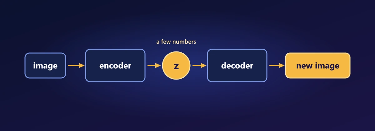
VAEs and GANs for Image Generation
What you'll learn: how to build models that create new images rather than label existing ones. We train a variational autoencoder (VAE) that invents handwritten digits, then open it up, and build a generative adversarial network (GAN), where two networks compete. The questions along the way lead into continuous probability in many dimensions: the multivariate Gaussian, the reparameterisation trick, the Kullback-Leibler (KL) divergence and its closed form, Jensen's inequality and the evidence lower bound, and the calculus behind the GAN's optimal discriminator.
Before you start: Lessons 1 to 13, especially probability densities and the normal distribution (Lesson 3), likelihood and the Bernoulli distribution (Lesson 4), backpropagation (Lesson 7) and PyTorch (Lesson 5).
Generate new handwritten digits
This trains a VAE on MNIST's 60,000 handwritten digits for a few epochs, then asks it to draw digits it has never seen, from random numbers:
import numpy as np
import torch
from torch import nn
import torch.nn.functional as F
from torch.utils.data import DataLoader
from torchvision import datasets, transforms
import matplotlib.pyplot as plt

mnist = datasets.MNIST("data", train=True, download=True, transform=transforms.ToTensor())
loader = DataLoader(mnist, batch_size=128, shuffle=True)

class VAE(nn.Module):
    def __init__(self, latent_dim=2):
        super().__init__()
        self.encoder = nn.Sequential(nn.Flatten(), nn.Linear(784, 400), nn.ReLU())
        self.mu = nn.Linear(400, latent_dim)
        self.log_var = nn.Linear(400, latent_dim)
        self.decoder = nn.Sequential(nn.Linear(latent_dim, 400), nn.ReLU(),
                                     nn.Linear(400, 784), nn.Sigmoid())

    def forward(self, x):
        h_ = self.encoder(x)
        mu, log_var = self.mu(h_), self.log_var(h_)
        z = mu + torch.exp(0.5 * log_var) * torch.randn_like(mu)    # the reparameterisation trick
        return self.decoder(z), mu, log_var

def vae_loss(x_hat, x, mu, log_var):
    reconstruction = F.binary_cross_entropy(x_hat, x.view(-1, 784), reduction="sum")
    kl = -0.5 * torch.sum(1 + log_var - mu ** 2 - log_var.exp())
    return (reconstruction + kl) / x.size(0)

torch.manual_seed(0)
vae = VAE()
optimizer = torch.optim.Adam(vae.parameters(), lr=1e-3)
for epoch in range(5):
    for x, _ in loader:
        x_hat, mu, log_var = vae(x)
        loss = vae_loss(x_hat, x, mu, log_var)
        optimizer.zero_grad(); loss.backward(); optimizer.step()
    print(f"epoch {epoch + 1}: loss {loss.item():.1f}")

vae.eval()
with torch.no_grad():
    grid = torch.linspace(-2.5, 2.5, 15)
    canvas = torch.zeros(15 * 28, 15 * 28)
    for i, yv in enumerate(grid):
        for j, xv in enumerate(grid):
            digit = vae.decoder(torch.stack([xv, yv]).view(1, 2)).view(28, 28)
            canvas[i * 28:(i + 1) * 28, j * 28:(j + 1) * 28] = digit
plt.figure(figsize=(8, 8)); plt.imshow(canvas.numpy(), cmap="gray"); plt.axis("off"); plt.show()epoch 1: loss 169.9 epoch 2: loss 162.4 epoch 3: loss 158.2 epoch 4: loss 148.1 epoch 5: loss 162.3
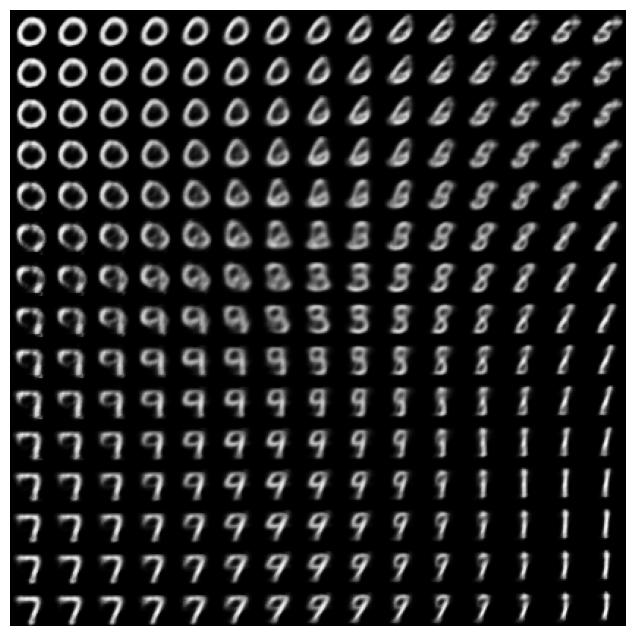
The picture is a map. Each tile is the decoder's drawing for one point (z₁, z₂) on a grid, and the digits morph smoothly into one another as you move across it: 0s blend into 6s, 7s into 1s and 9s. Every tile is new; none was in the training data. The whole space of digits has been organised onto a two-dimensional plane.
What just happened
A generative model learns the distribution of the data, so that it can sample new examples from it. Directly, that's hopeless: the space of 28 × 28 images has 784 dimensions, and almost all of it is static. Instead, the VAE learns a latent space: a simple distribution that's easy to sample from (here a 2-dimensional standard normal), together with a decoder network that maps each latent point z to an image. Sampling z and decoding it generates an image.
To learn that decoder, the VAE also learns an encoder that maps real images into the latent space, and trains both together like an autoencoder: encode a digit, decode it, and compare. A plain autoencoder (encoder → code → decoder, trained to reproduce its input) learns good compressions, but its codes can be scattered anywhere, with meaningless gaps between them, so decoding a random point usually gives garbage. The VAE makes the latent space smooth and gap-free with two changes, and each one raises a question about probability.
What is a Gaussian in many dimensions?
Question 1: the encoder doesn't output a point; it outputs μ and log σ² for a normal distribution. What is a normal distribution over a 2-dimensional, or 100-dimensional, space?
Lesson 3 met the one-dimensional normal density. The simplest many-dimensional version treats each coordinate as an independent normal variable with its own mean μⱼ and variance σⱼ². Independence means the joint density is the product of the individual densities (as with independent probabilities in Lesson 4), and a product of exponentials is the exponential of a sum:
Its density is a bell-shaped hill centred on the vector μ, stretched along each axis by σⱼ. The encoder turns each digit into such a hill, a small cloud of possible codes rather than one point, and the decoder must cope with any code drawn from the cloud. That alone pushes the clouds of similar digits to overlap, filling the gaps. We can check the product formula with SciPy's general multivariate normal:
from scipy.stats import multivariate_normal, norm

mu_ = np.array([1.0, -0.5]); sigma_ = np.array([0.7, 1.5]); z_ = np.array([0.4, 0.9])
product = norm.pdf(z_[0], mu_[0], sigma_[0]) * norm.pdf(z_[1], mu_[1], sigma_[1])
joint = multivariate_normal.pdf(z_, mean=mu_, cov=np.diag(sigma_ ** 2))
print(product, joint) # identical: independent coordinates multiply0.06791015313359586 0.06791015313359586
How can we backpropagate through a random sample?
Question 2: the decoder's input is sampled at random. How can a gradient flow back through "pick a random number" to the encoder's μ and σ?
It can't, directly: drawing a sample from N(μ, σ²) isn't a function of μ and σ that has a derivative. The reparameterisation trick moves the randomness out of the way. Sample noise ε from a fixed standard normal, which has no parameters, and compute z from it:
z is an ordinary differentiable function of μ and σ, with ε entering as an input like any other data. Backpropagation (Lesson 7) flows straight through, and autograd confirms the two derivatives:
mu_t = torch.tensor(2.0, requires_grad=True)
sigma_t = torch.tensor(0.5, requires_grad=True)
eps = torch.tensor(1.3)
z_t = mu_t + sigma_t * eps
z_t.backward()
print("dz/dmu =", mu_t.grad.item(), "  dz/dsigma =", sigma_t.grad.item(), "  epsilon =", eps.item())

samples = 2.0 + 0.5 * torch.randn(100_000)
print("mean", samples.mean().item(), " std", samples.std().item()) # about 2.0 and 0.5dz/dmu = 1.0 dz/dsigma = 1.2999999523162842 epsilon = 1.2999999523162842 mean 1.9996991157531738 std 0.4993535876274109
How different are two distributions?
Question 3: the loss includes a term that pulls every encoded cloud towards the standard normal N(0, I). How do we measure how far one distribution is from another?
The standard measure is the Kullback-Leibler divergence. In Lesson 4's language, −log p(z) is the surprise of seeing z under p. The KL divergence of q from p is the average extra surprise you'd experience if samples come from q but you expected p:
It is zero exactly when the two distributions are identical and positive otherwise (we'll see why in Question 4). It is not symmetric, KL(q ‖ p) ≠ KL(p ‖ q), so it isn't a true distance, but it is the natural one for comparing a model's distribution with another.
For a normal q = N(μ, σ²) and the standard normal p = N(0, 1), the expectation can be done by hand. Write out both log-densities from Question 1 and average them over q, using two facts about z ~ N(μ, σ²): E[(z − μ)²] = σ² (the definition of variance) and E[z²] = μ² + σ²:
Summed over the latent dimensions, that is exactly the kl line in the code: −½ Σ(1 + log σ² − μ² − σ²). Each dimension pays for moving its mean away from 0 (the μ² term) and for a variance different from 1 (σ² − 1 − log σ² is zero at σ = 1 and positive otherwise). A Monte Carlo estimate, averaging log q − log p over many samples, agrees:
def kl_closed_form(mu, log_var):
    return -0.5 * np.sum(1 + log_var - mu ** 2 - np.exp(log_var))

def kl_monte_carlo(mu, log_var, n=1_000_000, rng=np.random.default_rng(0)):
    sigma = np.exp(0.5 * log_var)
    z = mu + sigma * rng.normal(size=(n, len(mu)))
    log_q = np.sum(norm.logpdf(z, mu, sigma), axis=1)
    log_p = np.sum(norm.logpdf(z, 0, 1), axis=1)
    return np.mean(log_q - log_p)

mu_v, log_var_v = np.array([1.0, -0.5]), np.log(np.array([0.5, 2.0]))
print("closed form:", round(kl_closed_form(mu_v, log_var_v), 4), " Monte Carlo:", round(kl_monte_carlo(mu_v, log_var_v), 4))closed form: 0.875 Monte Carlo: 0.8763
Where does the VAE loss come from?
Question 4: reconstruction error plus a KL penalty looks like a sensible recipe. Is it more than that?
It is the negative of a lower bound on the log-likelihood of the data, which is what we'd really like to maximise. The model's probability of an image is an average over all codes, p(x) = ∫ p(x | z) p(z) dz, which can't be computed directly. Multiply and divide by the encoder's q(z | x) inside the integral, which turns it into an expectation under q:
Now we need Jensen's inequality. For a concave function, one that curves downwards like log, the function of an average is at least the average of the function: log E[Y] ≥ E[log Y]. (Picture any two points on the log curve: the straight chord between them lies below the curve, so averaging first and then taking the log gives the larger result.) Applying it:
This is the evidence lower bound (ELBO), and the VAE loss is exactly −ELBO. Pushing the bound up pushes log p(x) up with it. The same inequality, applied to −log, shows that a KL divergence can never be negative, which is the fact promised in Question 3.
And the reconstruction term? Treat each pixel as a Bernoulli variable (Lesson 4) whose probability of being "on" is the decoder's output. Then log p(x | z) is exactly the negative binary cross-entropy between the real pixels and the decoded ones, which is why the code uses F.binary_cross_entropy. Jensen's inequality is easy to check:
Y = np.random.default_rng(0).uniform(0.1, 5, 100_000)
print("log of the average:", round(np.log(Y.mean()), 4), " average of the log:", round(np.log(Y).mean(), 4))log of the average: 0.9353 average of the log: 0.6883
VAE samples tend to be slightly blurry. The pixel-wise reconstruction loss rewards hedging: when unsure where a stroke goes, a grey blend of the possibilities has a lower expected error than committing to one sharp stroke. GANs avoid that by learning what "realistic" means instead of writing it down.
Generative adversarial networks
A GAN (Ian Goodfellow and colleagues, 2014) has two networks. The generator G turns random noise z into an image G(z). The discriminator D looks at an image and outputs the probability that it is real. They are trained against each other: the discriminator to tell real from fake, the generator to fool it. Like a counterfeiter and a detective, each forces the other to improve, until the fakes are hard to tell from real images:
transform_gan = transforms.Compose([transforms.ToTensor(), transforms.Normalize((0.5,), (0.5,))])
gan_data = datasets.MNIST("data", train=True, download=True, transform=transform_gan)   # pixels in [-1, 1]
gan_loader = DataLoader(gan_data, batch_size=128, shuffle=True, drop_last=True)

latent_dim = 64
G = nn.Sequential(nn.Linear(latent_dim, 256), nn.LeakyReLU(0.2),
                  nn.Linear(256, 512), nn.LeakyReLU(0.2),
                  nn.Linear(512, 784), nn.Tanh())
D = nn.Sequential(nn.Linear(784, 512), nn.LeakyReLU(0.2),
                  nn.Linear(512, 256), nn.LeakyReLU(0.2),
                  nn.Linear(256, 1))                          # a logit: real or fake?

bce = nn.BCEWithLogitsLoss()
opt_G = torch.optim.Adam(G.parameters(), lr=2e-4, betas=(0.5, 0.999))
opt_D = torch.optim.Adam(D.parameters(), lr=2e-4, betas=(0.5, 0.999))

torch.manual_seed(0)
for epoch in range(10):
    for real, _ in gan_loader:
        real = real.view(-1, 784)
        ones, zeros = torch.ones(len(real), 1), torch.zeros(len(real), 1)

        fake = G(torch.randn(len(real), latent_dim))
        loss_D = bce(D(real), ones) + bce(D(fake.detach()), zeros)    # 1) discriminator step
        opt_D.zero_grad(); loss_D.backward(); opt_D.step()

        loss_G = bce(D(fake), ones)                                     # 2) generator step
        opt_G.zero_grad(); loss_G.backward(); opt_G.step()
    print(f"epoch {epoch + 1}: loss_D {loss_D.item():.3f}  loss_G {loss_G.item():.3f}")

with torch.no_grad():
    samples = G(torch.randn(16, latent_dim)).view(-1, 28, 28) * 0.5 + 0.5
fig, axes = plt.subplots(2, 8, figsize=(12, 3))
for ax, img in zip(axes.flat, samples):
    ax.imshow(img.numpy(), cmap="gray"); ax.axis("off")
plt.show()epoch 1: loss_D 0.904 loss_G 1.267 epoch 2: loss_D 0.660 loss_G 1.445 epoch 3: loss_D 0.395 loss_G 2.510 epoch 4: loss_D 0.467 loss_G 4.009 epoch 5: loss_D 1.006 loss_G 4.492 epoch 6: loss_D 0.590 loss_G 2.098 epoch 7: loss_D 0.323 loss_G 2.957 epoch 8: loss_D 0.397 loss_G 2.963 epoch 9: loss_D 0.444 loss_G 2.452 epoch 10: loss_D 0.514 loss_G 3.856
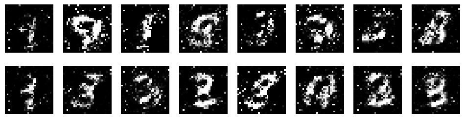
Don't expect the losses to fall steadily as in ordinary training: each network's progress makes the other's job harder, so in a healthy GAN they hover around each other. You judge a GAN by its samples, or with metrics such as the Fréchet Inception Distance. After ten epochs on a CPU, ours are still rough: speckled strokes in which some digits, such as 1s, 3s and 8s, are already readable and others aren't yet. There is no VAE-style blur, but sharpness takes longer. Train for more epochs, and replace these fully connected networks with convolutional ones (the DCGAN design), and the samples become clean digits.
What is the best possible discriminator?
Question 5: GAN training is a game. Where does it end up?
The game has one value function, which the discriminator tries to maximise and the generator to minimise:
where p_g is the distribution of the generator's images. For a fixed generator, the discriminator can choose D(x) separately at every x, so it maximises the integrand pointwise. At each x that means maximising a·log y + b·log(1 − y) over y between 0 and 1, with a = p_data(x) and b = p_g(x). Lesson 7's calculus: set the derivative to zero.
The best discriminator outputs the fraction of the probability at x that comes from real data. If the generator is perfect, p_g = p_data, then D* = ½ everywhere: a coin flip. Substituting D* back into V shows that the generator is minimising the Jensen-Shannon divergence between p_data and p_g (a symmetric relative of KL), whose minimum is zero, reached only when the two distributions match, where V = log ½ + log ½ = −log 4. We can verify on one-dimensional normal distributions standing in for real and generated data:
x = np.linspace(-10, 10, 200_001)
dx = x[1] - x[0]
p_data = norm.pdf(x, 0, 1)
for g_mean in [3.0, 1.0, 0.0]:                        # the generator approaches the data
    p_g = norm.pdf(x, g_mean, 1)
    D_star = p_data / (p_data + p_g)
    V = np.sum(p_data * np.log(D_star) + p_g * np.log(1 - D_star)) * dx
    print(f"generator mean {g_mean}: D*(0) = {D_star[100_000]:.3f}   V = {V:.4f}")
print("-log 4 =", round(-np.log(4), 4))generator mean 3.0: D*(0) = 0.989 V = -0.3327 generator mean 1.0: D*(0) = 0.622 V = -1.1635 generator mean 0.0: D*(0) = 0.500 V = -1.3863 -log 4 = -1.3863
Why does the generator use a different loss?
Question 6: in the code, the generator minimises bce(D(fake), ones), which is −log D(G(z)), not log(1 − D(G(z))) from the value function. Why the change?
Early in training, the generator's fakes are bad, the discriminator rejects them easily, and D(G(z)) ≈ 0. Look at the gradient each loss sends back to the discriminator's logit s, where D = σ(s). Using Lesson 7's σ' = σ(1 − σ): the derivative of log(1 − σ(s)) is −σ(s), which is about 0 when D is near 0. The generator gets no signal precisely when it most needs one. The derivative of −log σ(s) is −(1 − σ(s)), which is about −1 when D is near 0: a strong signal. Both losses push in the same direction (towards D(G(z)) = 1); the second just doesn't go quiet. This is called the non-saturating loss:
s = torch.tensor([-6.0, -3.0, 0.0, 3.0], requires_grad=True)      # discriminator logits for fakes
torch.log(1 - torch.sigmoid(s)).sum().backward()
print("D(G(z))                          ", torch.sigmoid(s).detach().numpy().round(3))
print("gradient of log(1 - D)  (minimax)", s.grad.numpy().round(3))
s.grad = None
(-torch.log(torch.sigmoid(s))).sum().backward()
print("gradient of -log D (non-saturating)", s.grad.numpy().round(3))D(G(z)) [0.002 0.047 0.5 0.953] gradient of log(1 - D) (minimax) [-0.002 -0.047 -0.5 -0.953] gradient of -log D (non-saturating) [-0.998 -0.953 -0.5 -0.047]
Why GANs are hard to train
GANs are temperamental. In mode collapse, the generator finds a few outputs that fool the discriminator and produces only those, ignoring the data's variety. Training can oscillate or diverge, and a discriminator that wins too easily starves the generator of gradient. A series of improvements tamed them: DCGAN's convolutional designs, Wasserstein GANs (a distance with smoother gradients than Jensen-Shannon), conditional GANs that take a label so you can request a particular digit, and StyleGAN, which generates photorealistic faces with control over pose, age and lighting.
VAEs and GANs compared
| VAE | GAN | |
|---|---|---|
| Training | Stable, one loss (−ELBO) | A two-player game, can be unstable |
| Samples | Smooth but often blurry | Sharp and realistic |
| Variety | Covers the whole data | Prone to mode collapse |
| Latent space | Smooth, with an encoder x → z | No encoder by default |
| Likelihood | A lower bound on log p(x) | None |
The two are often combined: VQ-VAE and VQ-GAN compress images into a compact latent space and model that space with a powerful generator, and Stable Diffusion runs its diffusion model inside the latent space of an autoencoder in exactly this way. Diffusion models are the subject of Lesson 15.
Summary
A generative model samples new data by decoding vectors from a simple latent distribution. A VAE's encoder outputs a diagonal multivariate Gaussian, a product of independent normals, for each input; the reparameterisation z = μ + σε makes sampling differentiable. Its loss is the negative ELBO: reconstruction (a Bernoulli log-likelihood per pixel) plus KL(q ‖ N(0, I)) = ½Σ(μ² + σ² − 1 − log σ²), and Jensen's inequality, log E[Y] ≥ E[log Y], proves it bounds log p(x). A GAN trains a generator against a discriminator; maximising pointwise gives D* = p_data/(p_data + p_g), the game's optimum has p_g = p_data with value −log 4, and the non-saturating loss −log D(G(z)) keeps gradients alive when the generator is losing.
Exercises
1. Show that the KL formula ½(μ² + σ² − 1 − log σ²) is zero only at μ = 0, σ = 1. (Hint: show that t − 1 − log t ≥ 0 with equality only at t = 1.)
2. Compute KL(N(0, 1) ‖ N(1, 4)) and KL(N(1, 4) ‖ N(0, 1)) by Monte Carlo. Are they equal? What does that tell you?
3. Use Jensen's inequality to prove that the arithmetic mean of positive numbers is at least their geometric mean.
4. Train the VAE with a 16-dimensional latent space instead of 2. How do reconstructions and samples change? Why can't you draw the map any more?
5. Make the GAN conditional: concatenate a one-hot digit label to the generator's noise and to the discriminator's input. Can you then ask for a specific digit?
6. Train the GAN with the original minimax generator loss, log(1 − D(G(z))). Compare the first epochs with the non-saturating version and explain what you see using Question 6.
7. Rebuild the GAN as a DCGAN: a generator of transposed convolutions that grows a 7 × 7 feature map to 28 × 28, and a convolutional discriminator like Lesson 9's classifier. Compare its samples after ten epochs with the fully connected GAN's.
Comments