Deep Learning Course · Lesson 13 of 16 · 28 min

Working with Large Language Models

Deepak Mishra, Senior Technology Lead at Incedo

What you'll learn: how large language models (LLMs) work and how to put them to use. We chat with a small instruction-tuned model, then open it up: next-token prediction, how text is generated, how a raw model becomes an assistant, and three ways to adapt one to your own problem: prompting, fine-tuning with LoRA, and retrieval-augmented generation (RAG). The questions along the way lead to the chain rule of probability, perplexity, entropy and temperature, and matrix rank, which explains why a tiny low-rank update can fine-tune a huge model.

Before you start: Lessons 1 to 12, especially softmax and temperature (Lesson 1), likelihood (Lesson 4), the SVD (Lesson 11) and the transformer (Lesson 12). A Colab GPU makes this lesson much faster but isn't required.

Talk to a language model

Qwen2.5-0.5B-Instruct is a small, openly available assistant model with half a billion parameters, small enough to run without a GPU:

import numpy as np
import torch
from torch import nn
from transformers import AutoTokenizer, AutoModelForCausalLM

chat_name = "Qwen/Qwen2.5-0.5B-Instruct"
chat_tokenizer = AutoTokenizer.from_pretrained(chat_name)
chat_model = AutoModelForCausalLM.from_pretrained(chat_name)

def ask(question, max_new_tokens=80):
    messages = [{"role": "user", "content": question}]
    inputs = chat_tokenizer.apply_chat_template(messages, add_generation_prompt=True,
                                                return_tensors="pt", return_dict=True)
    with torch.no_grad():
        out = chat_model.generate(**inputs, max_new_tokens=max_new_tokens, do_sample=False)
    return chat_tokenizer.decode(out[0, inputs["input_ids"].shape[1]:], skip_special_tokens=True)

print(ask("In two sentences, what is gradient descent?"))

Gradient descent is an optimization algorithm used to minimize a function by iteratively moving in the direction of steepest descent of the function's value, while gradually reducing the difference between successive iterations until convergence.

A coherent, relevant answer from a model that, underneath, does only one thing: given some text, it outputs a probability distribution over the next token. Everything an LLM does, from answering questions to writing code, is that operation repeated.

What just happened

The chat template wrapped the question in special tokens marking who is speaking. The model then predicted the next token, appended it, predicted the next, and so on, until it produced an end-of-turn token. It is the same GPT-style decoder from Lesson 12, with a causal mask, scaled up and trained in two stages. First, pretraining on trillions of tokens of text to predict the next token. Then, post-training on examples of helpful conversations, which turns a text continuer into an assistant. We'll take those in order.

Can every sentence be predicted one token at a time?

Question 1: a language model assigns a probability to any piece of text. How can predicting just the next token be enough to do that?

Because of the chain rule of probability. The definition of conditional probability, P(B | A) = P(A, B) / P(A), rearranges to P(A, B) = P(A) · P(B | A): the chance of both is the chance of the first times the chance of the second given the first. Apply it again and again to a sequence of tokens:

No approximation is involved: any probability distribution over sequences can be written this way. So a model that gets every next-token distribution right gets the probability of whole texts right. We can check the identity on a toy distribution over two-word sentences:

joint = {("the", "cat"): 0.3, ("the", "dog"): 0.2, ("a", "cat"): 0.1, ("a", "dog"): 0.4}
for (w1, w2), p_joint in joint.items():
    p_first = sum(p_ for (a, _), p_ in joint.items() if a == w1)          # P(w1)
    p_second_given_first = p_joint / p_first                               # P(w2 | w1)
    print(f"P({w1} {w2}) = {p_joint}   P({w1}) * P({w2}|{w1}) = {p_first * p_second_given_first:.2f}")

P(the cat) = 0.3   P(the) * P(cat|the) = 0.30
P(the dog) = 0.2   P(the) * P(dog|the) = 0.20
P(a cat) = 0.1   P(a) * P(cat|a) = 0.10
P(a dog) = 0.4   P(a) * P(dog|a) = 0.40

Training maximises the likelihood of the training text, which by Lesson 4 means minimising the average negative log-probability of each actual next token: the cross-entropy loss. With the causal mask, one forward pass computes the loss for every position in a sequence at once.

How good is a language model?

Question 2: the loss is an average negative log-probability. Is there a more intuitive way to read it?

Exponentiate it. Perplexity is e raised to the average negative log-probability per token:

If a model were choosing uniformly among k equally likely tokens at every step, each log-probability would be log(1/k), and the perplexity would be exactly k. So perplexity is the model's effective number of choices per token: a perplexity of 20 means the model is, on average, as uncertain as if it were picking among 20 equally likely tokens. Lower is better. Compare a normal sentence with the same words shuffled, using GPT-2:

gpt2_tok = AutoTokenizer.from_pretrained("gpt2")
gpt2 = AutoModelForCausalLM.from_pretrained("gpt2")

def perplexity(text):
    ids = gpt2_tok(text, return_tensors="pt").input_ids
    with torch.no_grad():
        loss = gpt2(ids, labels=ids).loss          # average next-token cross-entropy
    return torch.exp(loss).item()

sentence = "The cat sat on the mat and looked out of the window at the rain."
shuffled = "Rain mat window the of looked sat the at the cat and out on the."
print(f"normal:   perplexity {perplexity(sentence):8.1f}")
print(f"shuffled: perplexity {perplexity(shuffled):8.1f}")
print("uniform guessing over GPT-2's vocabulary:", gpt2_tok.vocab_size)

normal:   perplexity     22.1
shuffled: perplexity   1013.3
uniform guessing over GPT-2's vocabulary: 50257

Generating text

Generation repeats: compute the next-token distribution, choose a token, append it. How you choose matters. Greedy decoding always takes the most likely token, which is predictable and tends to repeat itself. Sampling picks at random according to the probabilities, with a few controls: temperature T divides the logits before the softmax (Lesson 1), top-k keeps only the k most likely tokens, and top-p keeps the smallest set of tokens whose probabilities add up to p.

How random is a distribution?

Question 3: temperature makes generation "more random". Can we measure randomness?

Yes, with entropy, the average surprise of a distribution. The surprise of an outcome with probability p is −log p (Lesson 4's loss is exactly the surprise of the right answer), and entropy is its expected value:

Perplexity and entropy are related: e^H is the effective number of choices of a distribution. As the temperature rises, the softmax flattens and the entropy climbs towards its maximum; as it falls, the distribution sharpens and the entropy drops towards zero:

def entropy(probs):
    probs = probs[probs > 0]
    return -(probs * probs.log()).sum().item()

ids = gpt2_tok("The capital of France is", return_tensors="pt").input_ids
with torch.no_grad():
    logits = gpt2(ids).logits[0, -1]

for T in [0.2, 0.7, 1.0, 1.5]:
    probs = torch.softmax(logits / T, dim=0)
    H = entropy(probs)
    print(f"T = {T}: entropy {H:5.2f} nats, effective choices e^H = {np.exp(H):8.1f}")
print("maximum possible entropy, log(50257) =", round(np.log(50257), 2))

T = 0.2: entropy  0.53 nats, effective choices e^H =      1.7
T = 0.7: entropy  3.55 nats, effective choices e^H =     34.9
T = 1.0: entropy  6.00 nats, effective choices e^H =    402.8
T = 1.5: entropy  8.48 nats, effective choices e^H =   4815.8
maximum possible entropy, log(50257) = 10.82

Here is what that does to the ten most likely next tokens:

PythonCopy

import matplotlib.pyplot as plt

top = torch.topk(logits, 10).indices
labels = [gpt2_tok.decode([int(t)]) for t in top]
fig, axes = plt.subplots(1, 3, figsize=(15, 3.8), sharey=True)
for ax, T in zip(axes, [0.2, 1.0, 1.5]):
    probs = torch.softmax(logits / T, dim=0)
    ax.bar(range(10), probs[top].numpy())
    ax.set_xticks(range(10), labels, rotation=60)
    ax.set_title(f"T = {T}")
axes[0].set_ylabel("probability")
plt.show()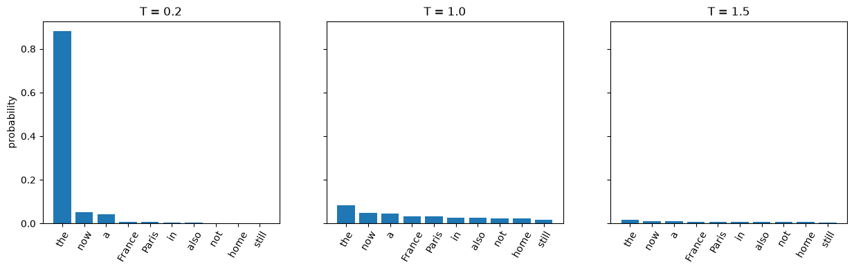

Output

A temperature near 0 approaches greedy decoding; a high temperature lets in thousands of unlikely tokens, which is where nonsense comes from. Top-p adapts to the situation: when the model is sure, a few tokens reach p and only those are allowed; when it's unsure, many are.

From text predictor to assistant

A pretrained model only continues text. Ask it a question and it may continue with more questions, because that's what text on the web often does. Post-training turns it into an assistant, in two common stages. Supervised fine-tuning (instruction tuning) trains on many examples of prompts with high-quality responses, using the same next-token loss. Preference optimisation then shows the model pairs of responses, one preferred by people, and nudges it to make preferred responses more likely, either with reinforcement learning from human feedback (RLHF) or with direct preference optimisation (DPO), which turns the preference comparisons into a simple classification-style loss. This is also where models learn to decline harmful requests and to say when they're unsure.

Large models also show in-context learning: given a few examples of a task in the prompt, they perform it without any change to their weights. That makes prompting the first, cheapest way to adapt an LLM.

reviews = ["Setup took two minutes and it just works.", "The screen cracked on day two.",
           "Customer service never replied to my emails.", "Honestly the best headphones I've owned."]
for review in reviews:
    prompt = f"""Classify the sentiment of each review as positive or negative. Answer with one word.
Review: The battery lasts all day. Sentiment: positive
Review: It broke after one week. Sentiment: negative
Review: {review} Sentiment:"""
    print(f"{ask(prompt, max_new_tokens=5):10s} {review}")

negative   Setup took two minutes and it just works.
negative   The screen cracked on day two.
negative   Customer service never replied to my emails.
positive   Honestly the best headphones I've owned.

From two examples and no training, the model labels three of the four reviews correctly. It calls the two-minute setup negative, perhaps misled by the word "just". Mistakes like this are typical of a model with half a billion parameters: in-context learning becomes far more reliable as models grow. When a small model's prompting isn't reliable enough, or a large model is too expensive to run, the next step is to change the weights.

Fine-tuning a model on your own data

Fine-tuning does that: continue training a pretrained model on your own labelled examples. Here we fine-tune DistilBERT, a small BERT (Lesson 11), to tell apart newsgroup posts about space and about medicine. Updating all of its 66 million weights works, but there's a cheaper way, and to see why it works we need one more idea from linear algebra.

Why can a small update be enough?

Question 4: fine-tuning changes each weight matrix W to W + ΔW. Does ΔW really need as many numbers as W?

The rank of a matrix is the number of independent directions it can produce: the dimension of the space its outputs live in. A d × d matrix can have rank up to d. But a product B·A, with B of shape d × r and A of shape r × d, has rank at most r, because every output BAx = B(Ax) passes through the r-dimensional bottleneck Ax. Such a product needs only 2dr numbers instead of d².

Lesson 11's SVD says how much is lost by forcing a matrix to have low rank: the best rank-r approximation keeps the r largest singular values, and the error comes only from the ones dropped. If the singular values fall off quickly, a low-rank matrix captures almost everything. Researchers found that the weight changes made by fine-tuning have exactly this property: they have low intrinsic rank, because adapting to a narrow task only needs to adjust a few directions.

torch.manual_seed(0)
d = 256
# A "fine-tuning update" whose importance is concentrated in a few directions
U, _ = torch.linalg.qr(torch.randn(d, d))
V, _ = torch.linalg.qr(torch.randn(d, d))
singular_values = 10 * 0.5 ** torch.arange(d, dtype=torch.float32)       # quickly decaying
delta_W = U @ torch.diag(singular_values) @ V.T

for r in [1, 4, 8, 16]:
    Uw, S, Vh = torch.linalg.svd(delta_W)
    approx = Uw[:, :r] @ torch.diag(S[:r]) @ Vh[:r]
    error = (delta_W - approx).norm() / delta_W.norm()
    print(f"rank {r:2d}: {2 * d * r:6,d} numbers instead of {d * d:,}   relative error {error:.1e}")
print("rank of a product B @ A with r = 8:", torch.linalg.matrix_rank(torch.randn(d, 8) @ torch.randn(8, d)).item())

rank  1:    512 numbers instead of 65,536   relative error 5.0e-01
rank  4:  2,048 numbers instead of 65,536   relative error 6.3e-02
rank  8:  4,096 numbers instead of 65,536   relative error 3.9e-03
rank 16:  8,192 numbers instead of 65,536   relative error 1.6e-05
rank of a product B @ A with r = 8: 8

LoRA: low-rank adaptation

LoRA (Hu et al., 2021) builds this into fine-tuning. It freezes every original weight matrix W and learns only a low-rank correction:

A starts random and B starts at zero, so at the beginning W' = W exactly and the model behaves as before; training then grows the correction. With r = 8, each adapted 768 × 768 matrix trains 2 · 768 · 8 = 12,288 numbers instead of 589,824, about 2% of its weights, so fine-tuning fits on small GPUs, and one base model can carry many small task-specific adapters. Here is LoRA from scratch, injected into DistilBERT's attention query and value projections:

from sklearn.datasets import fetch_20newsgroups
from transformers import AutoModelForSequenceClassification

class LoRALinear(nn.Module):
    def __init__(self, base, r=8, alpha=16):
        super().__init__()
        self.base = base
        for p_ in self.base.parameters():
            p_.requires_grad = False                                 # freeze W and its bias
        self.A = nn.Parameter(torch.randn(r, base.in_features) * 0.01)
        self.B = nn.Parameter(torch.zeros(base.out_features, r))     # starts at zero: W' = W
        self.scale = alpha / r

    def forward(self, x):
        return self.base(x) + (x @ self.A.T @ self.B.T) * self.scale

name = "distilbert-base-uncased"
tok = AutoTokenizer.from_pretrained(name)
clf = AutoModelForSequenceClassification.from_pretrained(name, num_labels=2)
for p_ in clf.distilbert.parameters():
    p_.requires_grad = False                                         # freeze the whole backbone
for block in clf.distilbert.transformer.layer:
    block.attention.q_lin = LoRALinear(block.attention.q_lin)
    block.attention.v_lin = LoRALinear(block.attention.v_lin)

trainable = sum(p_.numel() for p_ in clf.parameters() if p_.requires_grad)
total = sum(p_.numel() for p_ in clf.parameters())
print(f"training {trainable:,} of {total:,} parameters ({trainable / total:.2%})")

cats = ["sci.space", "sci.med"]
train = fetch_20newsgroups(subset="train", categories=cats, remove=("headers", "footers", "quotes"))
test = fetch_20newsgroups(subset="test", categories=cats, remove=("headers", "footers", "quotes"))

def encode(texts):
    return tok(texts, truncation=True, max_length=128, padding=True, return_tensors="pt")

def test_accuracy(n=300):
    clf.eval()
    batch = encode(test.data[:n])
    with torch.no_grad():
        preds = clf(**batch).logits.argmax(1)
    return (preds == torch.tensor(test.target[:n])).float().mean().item()

print(f"before fine-tuning: test accuracy {test_accuracy():.1%}")
optimizer = torch.optim.AdamW([p_ for p_ in clf.parameters() if p_.requires_grad], lr=1e-3)
clf.train()
torch.manual_seed(0)
order = torch.randperm(len(train.data))[:480]
for start in range(0, len(order), 16):
    idx = order[start:start + 16].tolist()
    batch = encode([train.data[i] for i in idx])
    labels = torch.tensor(train.target[idx])
    loss = clf(**batch, labels=labels).loss
    optimizer.zero_grad(); loss.backward(); optimizer.step()
print(f"after fine-tuning on 480 posts: test accuracy {test_accuracy():.1%}")

training 739,586 of 67,102,466 parameters (1.10%)
before fine-tuning: test accuracy 53.3%
after fine-tuning on 480 posts: test accuracy 93.3%

Before fine-tuning, the new classification head is random and accuracy is near a coin flip. After one pass over 480 posts, training about 1% of the parameters, the model separates space from medicine with high accuracy. In practice you would use the peft library, which applies LoRA to any Hugging Face model in a few lines, but there is nothing more to it than the class above.

Retrieval-augmented generation

An LLM only knows what was in its training data, which is frozen at some date and doesn't include your private documents. Asked about them, it may invent a plausible-sounding answer, a hallucination: it is producing likely text, not checked facts (Lesson 2's GPT-2 put " the" ahead of " Paris" for the same reason). Retrieval-augmented generation fixes this by finding relevant documents first, with the semantic search of Lesson 2, and putting them in the prompt, so the model answers from the evidence and can cite it:

from sentence_transformers import SentenceTransformer

documents = [
    "Our refund policy allows returns within 30 days of delivery with the original receipt.",
    "Support is available Monday to Friday, 9am to 6pm IST, by email at help@example.com.",
    "Premium plans include priority support and a dedicated account manager.",
    "Orders above 2,000 rupees ship free anywhere in India.",
]
encoder = SentenceTransformer("all-MiniLM-L6-v2")
doc_vectors = encoder.encode(documents, normalize_embeddings=True)

def rag_answer(question, k=2):
    q = encoder.encode(question, normalize_embeddings=True)
    top = np.argsort(-(doc_vectors @ q))[:k]                  # cosine similarity (Lesson 2)
    context = "\n".join(f"- {documents[i]}" for i in top)
    prompt = (f"Answer the question using only the information below. "
              f"If it isn't there, say you don't know.\n{context}\n\nQuestion: {question}")
    return ask(prompt, max_new_tokens=120)

print(rag_answer("Can I return something I bought three weeks ago?"))
print(rag_answer("What is the CEO's name?"))

Yes, you can return something you purchased three weeks ago. The refund policy allows for returns within 30 days of delivery with the original receipt.
I'm sorry, but I do not have enough information to determine the CEO's name based solely on the provided details. The text does mention that the company has a premium plan with priority support and a dedicated account manager, but it doesn't specify who this person is or their name. Without additional context about the CEO's role or identity, I cannot provide an accurate answer to your question.

The first answer comes from the refund policy; for the second, the documents contain nothing relevant and the prompt tells the model to say so. RAG is the standard way to build assistants over company documents: it keeps answers current (update the documents, not the model) and checkable (show the sources).

Scale

Why have LLMs improved so dramatically? Mostly scale. Research on scaling laws found that the loss falls smoothly and predictably as parameters, training data and compute grow together. A transformer block has about 12 · d_model² parameters (about 4d² in attention and 8d² in the feed-forward layer), so with d_model = 768 and 12 blocks, plus the token embedding table, GPT-2 has about 124 million. Today's frontier models have hundreds of billions of parameters, trained on trillions of tokens:

d, layers, vocab = 768, 12, 50257
estimate = 12 * d * d * layers + vocab * d
print(f"rule of thumb: {estimate / 1e6:.0f}M   GPT-2 actual: {sum(p_.numel() for p_ in gpt2.parameters()) / 1e6:.0f}M")

rule of thumb: 124M   GPT-2 actual: 124M

Summary

An LLM is a decoder-only transformer that outputs a distribution over the next token; by the chain rule of probability, P(x₁, …, xₙ) = Π P(xₜ | x₍<ₜ₎), so getting every next token right means modelling whole texts. It is trained by minimising cross-entropy, and perplexity, the exponential of that loss, is its effective number of choices per token. Generation samples from the distribution, with temperature controlling its entropy H = −Σ p log p. Instruction tuning and preference optimisation turn a text predictor into an assistant. Adapt a model by prompting (including in-context examples), by fine-tuning, where LoRA's W + BA exploits the low rank of fine-tuning updates to train about 1% of the weights, or by retrieval-augmented generation, which grounds answers in retrieved documents and reduces hallucination.

Exercises

1. Extend the chain-rule check to three-word sentences: build a joint distribution and verify P(a, b, c) = P(a)·P(b | a)·P(c | a, b).

2. Show that the entropy of a uniform distribution over k outcomes is log k, and that its perplexity is k.

3. Compute the perplexity of GPT-2 on a paragraph of English, a paragraph of code, and a paragraph in another language. Explain the differences.

4. Prove that rank(BA) ≤ r when B is d × r and A is r × d. Then check that LoRA's update really has rank at most 8 after training.

5. Repeat the fine-tuning with r = 1, 2, 8 and 32. How do accuracy and the number of trainable parameters change?

6. Add ten documents about a topic you know to the RAG example and ask questions that need two documents at once. When does retrieval fail, and how could you fix it?