Deep Learning CourseLesson 12 of 16 26 min
Attention and Transformers
What you'll learn: how the transformer works, the architecture behind every large language model and much of modern AI. We start by looking inside a real one, GPT-2, to see which words attend to which. Then we build every piece in PyTorch: scaled dot-product attention, self-attention, multi-head attention, positional encoding, the transformer block and the causal mask. The questions along the way lead to the variance of a dot product (why we divide by √d_k), attention as an expected value, why attention on its own ignores word order, and why sine waves encode position as a rotation.
Before you start: Lessons 1 to 11, especially dot products (Lesson 2), variance of sums (Lessons 3 and 6), matrices (Lesson 5), skip connections (Lesson 9) and the limits of RNNs (Lesson 10).
Look inside a transformer
GPT-2 is a 12-layer transformer. Ask it to return its attention weights, and you can see, for every word, how much it looks at each earlier word:
import numpy as np
import torch
from torch import nn
from transformers import AutoTokenizer, AutoModel

tokenizer = AutoTokenizer.from_pretrained("gpt2")
gpt2 = AutoModel.from_pretrained("gpt2", attn_implementation="eager")

sentence = "The animal didn't cross the street because it was too tired"
inputs = tokenizer(sentence, return_tensors="pt")
with torch.no_grad():
    attentions = gpt2(**inputs, output_attentions=True).attentions   # one tensor per layer

tokens = [tokenizer.decode([t]) for t in inputs["input_ids"][0]]
it = tokens.index(" it")
print(len(attentions), "layers;", attentions[0].shape[1], "heads per layer")

# For each head in layer 5, which earlier word does " it" attend to most (ignoring the first token)?
layer = attentions[4][0]                       # (heads, tokens, tokens)
for head in range(12):
    weights = layer[head, it, 1:it + 1]
    best = int(weights.argmax()) + 1
print(f"head {head:2d}: ' it' attends most to {tokens[best]!r:12} ({weights.max():.2f})")12 layers; 12 heads per layer head 0: ' it' attends most to ' it' (0.10) head 1: ' it' attends most to ' because' (0.73) head 2: ' it' attends most to ' because' (0.06) head 3: ' it' attends most to ' animal' (0.85) head 4: ' it' attends most to ' it' (0.06) head 5: ' it' attends most to "'t" (0.06) head 6: ' it' attends most to ' animal' (0.16) head 7: ' it' attends most to ' it' (0.53) head 8: ' it' attends most to ' because' (0.04) head 9: ' it' attends most to "'t" (0.27) head 10: ' it' attends most to ' because' (0.05) head 11: ' it' attends most to ' because' (1.00)
Different heads look at different words. Several attend mostly to "because", the word just before "it"; a couple attend to "it" itself; and head 3 puts 85% of its attention on "animal", the word "it" refers to. Nobody told it about pronouns: each head has learned its own way of gathering context. This lesson explains what a head computes.
The whole attention pattern of that head, as a heatmap. Each row is a token, and its row shows how that token's attention is shared among itself and the tokens before it:
import matplotlib.pyplot as plt

plt.figure(figsize=(7, 6))
plt.imshow(layer[3].numpy(), cmap="Blues")
plt.xticks(range(len(tokens)), tokens, rotation=90); plt.yticks(range(len(tokens)), tokens)
plt.xlabel("attends to"); plt.ylabel("token"); plt.title("GPT-2 layer 5, head 3")
plt.colorbar(); plt.show()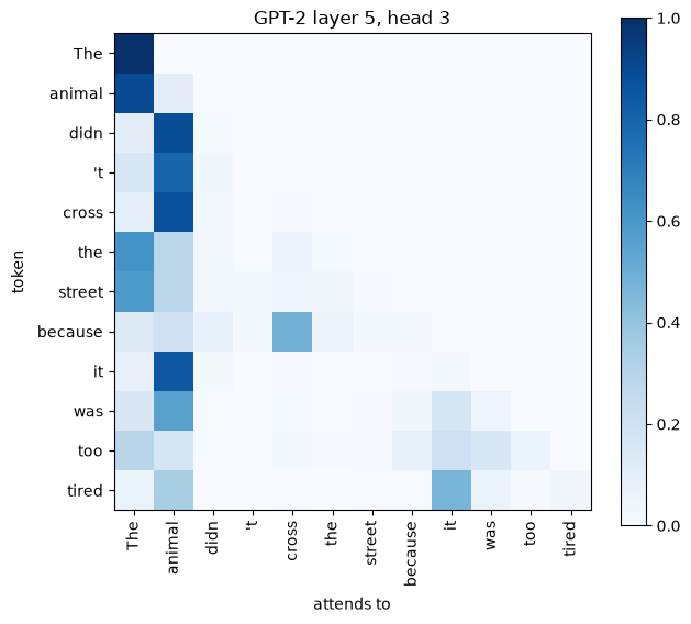
Look at the column under "animal": "it" is not the only token attending to it. "didn", "cross" and "was" do too. This head seems to track the subject of the sentence in general, and pointing "it" at the animal falls out of that. Reading a meaning into one head from one sentence is easy; checking the pattern across many sentences is the real test, which Exercise 6 starts.
What just happened
Lesson 10 ended with two problems of RNNs: they read one word at a time, which can't be parallelised, and information from early words has to survive being passed along every step. Attention solves both. Every word can look directly at every other word, however far apart, and all those comparisons are computed at once as one matrix multiplication. The 2017 paper that introduced the transformer was titled "Attention Is All You Need", and the rest of the architecture is support for that one operation.
Attention as a soft lookup
A dictionary lookup compares your query with every key, finds the exact match, and returns its value. Attention does a soft version: compare a query vector with every key vector, score how well each matches, and return a weighted average of the values, with better matches weighted more. Stacking the queries, keys and values as rows of matrices Q, K and V:
def attention(Q, K, V, mask=None):
    d_k = Q.shape[-1]
    scores = Q @ K.transpose(-2, -1) / d_k ** 0.5
    if mask is not None:
        scores = scores.masked_fill(~mask, float("-inf"))   # blocked: weight exactly 0
    weights = torch.softmax(scores, dim=-1)
    return weights @ V, weights

Q = torch.tensor([[1.0, 0.0]])
K = torch.tensor([[1.0, 0.0], [0.0, 1.0], [0.7, 0.7]])    # matches, unrelated, partly matches
V = torch.tensor([[10.0, 0.0], [0.0, 10.0], [5.0, 5.0]])
out, w = attention(Q, K, V)
print("weights:", w.numpy().round(3), " output:", out.numpy().round(2))

reference = nn.functional.scaled_dot_product_attention(Q, K, V)
print("matches PyTorch's built-in:", torch.allclose(out, reference))weights: [[0.434 0.214 0.351]] output: [[6.1 3.9]] matches PyTorch's built-in: True
Why divide by √d_k?
Question 1: the scores are divided by the square root of the key dimension. Why that number?
Think about the size of a dot product q · k = Σ qᵢkᵢ over d_k dimensions, when the entries are independent with mean 0 and variance 1. Each product qᵢkᵢ has variance 1 (Lesson 6: the variance of a product of independent zero-mean variables is the product of their variances), and variances of independent terms add (Lesson 3). So q · k has variance d_k, and standard deviation √d_k. With d_k = 64, raw scores are typically around ±8.
That matters because of what softmax does with large scores. Lesson 1 showed that only the differences between scores matter, and that big differences push nearly all the probability onto one option. A softmax that is that sure has almost no gradient: if one weight is about 1 and the rest about 0, nudging the scores barely changes anything, because the derivative of a softmax weight p with respect to its own score is p(1 − p), which is close to zero when p is near 0 or 1. Training stalls. Dividing by √d_k brings the scores' standard deviation back to 1:
torch.manual_seed(0)
for d_k in [4, 64, 512]:
    q, k = torch.randn(10_000, d_k), torch.randn(10_000, d_k)
    dots = (q * k).sum(dim=1)
    print(f"d_k = {d_k:3d}: std of q.k = {dots.std():6.2f}   after / sqrt(d_k) = {(dots / d_k ** 0.5).std():.2f}")

scores = torch.randn(10) * 8                       # unscaled scores for d_k = 64
for name, s in [("unscaled", scores), ("scaled", scores / 8)]:
    p_ = torch.softmax(s, dim=0)
print(f"{name:9s}: largest weight {p_.max():.3f}, its gradient p(1-p) = {(p_.max() * (1 - p_.max())):.4f}")d_k = 4: std of q.k = 1.99 after / sqrt(d_k) = 1.00 d_k = 64: std of q.k = 8.01 after / sqrt(d_k) = 1.00 d_k = 512: std of q.k = 22.49 after / sqrt(d_k) = 0.99 unscaled : largest weight 0.999, its gradient p(1-p) = 0.0013 scaled : largest weight 0.327, its gradient p(1-p) = 0.2201
What is the output, statistically?
Question 2: the attention weights for one query sum to 1. What does that make the output?
Non-negative weights that sum to 1 are a probability distribution over the keys (Lesson 1), so the output Σⱼ wⱼVⱼ is an expected value: the average value you'd get if you picked key j with probability wⱼ. Each output is a blend of the values, lying "between" them, pulled towards the values whose keys best matched the query. In the example above, the query matched key 0 best, so the output (6.1, 3.9) is pulled towards V₀ = (10, 0). Attention doesn't copy one value; it computes an expected value under a distribution that the query chooses.
Self-attention
In self-attention, the queries, keys and values all come from the same sequence. Every token's embedding is projected three ways by learned matrices:
The query says what a token is looking for, the key what it offers, and the value what it passes on. In "The animal didn't cross the street because it was too tired", the query for "it" can match the key of "animal", so the new vector for "it" absorbs information about the animal. Change "tired" to "wide" and a trained model shifts its attention to "street". Every pair of tokens is connected directly, in one step, whatever the distance between them.
torch.manual_seed(0)
n_tokens, d_model = 5, 16
X = torch.randn(n_tokens, d_model)
W_Q, W_K, W_V = (torch.randn(d_model, d_model) / d_model ** 0.5 for _ in range(3))
out, weights = attention(X @ W_Q, X @ W_K, X @ W_V)
print(weights.numpy().round(2))     # row i: how much token i attends to each token
print(out.shape) # one new vector per token[[0.12 0.46 0.21 0.13 0.08] [0.21 0.12 0.1 0.37 0.2 ] [0.36 0.09 0.33 0.06 0.16] [0.02 0.93 0.05 0. 0. ] [0.23 0.47 0.21 0.04 0.05]] torch.Size([5, 16])
Multi-head attention
A word relates to its sentence in several ways at once: its subject, the noun an adjective describes, the previous word, a pronoun's referent. One attention pattern can capture only one of these. Multi-head attention runs h attention operations in parallel, each on its own slice of d_model / h dimensions with its own projections, then joins the results and mixes them with one more matrix W_O. That's the 12 heads per layer we saw in GPT-2:
def multi_head_attention(X, W_Q, W_K, W_V, W_O, n_heads, mask=None):
    n, d_model = X.shape
    d_k = d_model // n_heads
    split = lambda M: M.reshape(n, n_heads, d_k).transpose(0, 1)    # (heads, tokens, d_k)
    Q, K, V = split(X @ W_Q), split(X @ W_K), split(X @ W_V)
    heads, _ = attention(Q, K, V, mask)                              # all heads at once
    return heads.transpose(0, 1).reshape(n, d_model) @ W_O

W_O = torch.randn(d_model, d_model) / d_model ** 0.5
print(multi_head_attention(X, W_Q, W_K, W_V, W_O, n_heads=4).shape) # same shape as Xtorch.Size([5, 16])
Does attention know the order of the words?
Question 3: "dog bites man" and "man bites dog" contain the same tokens. Can self-attention tell them apart?
Not on its own. Shuffle the input rows with a permutation P (a matrix that reorders rows). The scores become (PQ)(PK)ᵀ = P(QKᵀ)Pᵀ, which is the same scores with rows and columns reordered; softmax works row by row, so the weights are reordered the same way; and multiplying by PV gives P times the original output. Self-attention is permutation-equivariant: shuffle the input and you get the same outputs, shuffled. It treats the sentence as a bag of words.
perm = torch.tensor([3, 0, 4, 1, 2])
out_original = multi_head_attention(X, W_Q, W_K, W_V, W_O, n_heads=4)
out_shuffled = multi_head_attention(X[perm], W_Q, W_K, W_V, W_O, n_heads=4)
print("shuffled input gives shuffled output:", torch.allclose(out_shuffled, out_original[perm], atol=1e-5))shuffled input gives shuffled output: True
So position has to be added to the input. The original transformer added a positional encoding to each token's embedding before the first layer, built from sine and cosine waves of different frequencies:
Why sines and cosines?
Question 4: why encode a position with waves, rather than just the number pos?
Raw numbers grow without bound and would swamp the embeddings. Waves stay between −1 and 1, and using many frequencies, from fast to very slow like the hands of a clock, gives every position a unique pattern. But the real reason is subtler: with sines and cosines, moving k positions along is a rotation. Each pair of dimensions (sin(pos·ω), cos(pos·ω)) is a point on a circle at angle pos·ω. The angle-addition formulas say what happens at pos + k:
The matrix depends only on the offset k, not on pos. So "three positions later" is the same linear map (a rotation) wherever you are in the sentence, which makes relative positions easy for the linear projections W_Q and W_K to use. Many modern LLMs take this idea further with rotary position embeddings (RoPE), which rotate the queries and keys directly.
def positional_encoding(n_positions, d_model):
    pos = torch.arange(n_positions).float()[:, None]
    omega = 1 / 10000 ** (torch.arange(0, d_model, 2).float() / d_model)
    pe = torch.zeros(n_positions, d_model)
    pe[:, 0::2] = torch.sin(pos * omega)
    pe[:, 1::2] = torch.cos(pos * omega)
    return pe

pe = positional_encoding(50, 16)
w0, k = 1.0, 3                                     # first frequency (omega = 1), offset of 3
R = torch.tensor([[np.cos(k * w0), np.sin(k * w0)], [-np.sin(k * w0), np.cos(k * w0)]], dtype=torch.float32)
for pos in [0, 10, 40]:
print(f"pos {pos:2d}: rotating gives position {pos + k}:", torch.allclose(R @ pe[pos, :2], pe[pos + k, :2], atol=1e-5))pos 0: rotating gives position 3: True pos 10: rotating gives position 13: True pos 40: rotating gives position 43: True
The transformer block
A transformer is a stack of identical blocks. Each block has two sub-layers: multi-head self-attention, where tokens exchange information, and a feed-forward network (Lesson 6) applied to each token separately, where each token processes what it gathered. Each sub-layer sits on a residual connection (Lesson 9) and is preceded by layer normalisation:
The residual connections give gradients a direct path through dozens of blocks, exactly as in ResNet. Layer normalisation is Lesson 8's batch normalisation turned sideways: it standardises across the features of each token rather than across the batch, so it behaves the same for any batch size or sequence length.
class TransformerBlock(nn.Module):
    def __init__(self, d_model, n_heads, d_ff):
        super().__init__()
        self.attn = nn.MultiheadAttention(d_model, n_heads, batch_first=True)
        self.ff = nn.Sequential(nn.Linear(d_model, d_ff), nn.ReLU(), nn.Linear(d_ff, d_model))
        self.norm1, self.norm2 = nn.LayerNorm(d_model), nn.LayerNorm(d_model)

    def forward(self, x, mask=None):
        h_ = self.norm1(x)
        x = x + self.attn(h_, h_, h_, attn_mask=mask, need_weights=False)[0]
        return x + self.ff(self.norm2(x))

block = TransformerBlock(d_model=64, n_heads=4, d_ff=256)
tokens = torch.randn(2, 10, 64) + positional_encoding(10, 64)    # batch of 2, 10 tokens each
print(block(tokens).shape)                                        # the shape never changes
print("parameters per block:", sum(p_.numel() for p_ in block.parameters()))torch.Size([2, 10, 64]) parameters per block: 49984
The causal mask
The original transformer had an encoder, which reads the input with every token attending to every other, and a decoder, which generates output. BERT kept only the encoder, for understanding tasks. GPT and most LLMs keep only the decoder, for generation.
A generator writes left to right, so while training it must not see the future, or predicting the next word would be trivial. A causal mask sets every score above the diagonal to −∞ before the softmax, and e^(−∞) = 0, so each token attends only to itself and earlier tokens:
n = 5
causal = torch.tril(torch.ones(n, n, dtype=torch.bool))     # lower triangle = allowed
_, w = attention(torch.randn(n, 8), torch.randn(n, 8), torch.randn(n, 8), mask=causal)
print(w.numpy().round(2)) # zeros above the diagonal[[1. 0. 0. 0. 0. ] [0.94 0.06 0. 0. 0. ] [0.2 0.73 0.07 0. 0. ] [0.03 0.8 0.01 0.16 0. ] [0.05 0.57 0. 0.25 0.12]]
Thanks to the mask, one forward pass over a sentence trains the model to predict every next word in it at once, which is a big part of why transformers train so efficiently.
The cost of attention
Every token is compared with every other, so attention's compute and memory grow with the square of the sequence length: twice the context costs four times as much. Techniques such as FlashAttention (computing attention in GPU-friendly tiles without storing the full table of scores), sliding-window attention, and caching the keys and values of earlier tokens during generation are what make long context windows practical.
Summary
Attention is a soft lookup: Attention(Q, K, V) = softmax(QKᵀ/√d_k)V, where each output is an expected value of the values under a distribution chosen by the query. The dot product of random d_k-dimensional vectors has variance d_k, and dividing by √d_k keeps the softmax out of its saturated, gradient-free regime. Self-attention computes Q, K and V from the same tokens, multi-head attention runs several patterns in parallel, and since attention is permutation-equivariant, positions are added with sinusoidal encodings, whose angle-addition structure turns an offset into a rotation. A transformer block combines attention and a feed-forward network with residual connections and layer normalisation, and a causal mask turns it into a left-to-right generator. Lesson 13 turns this generator into a large language model.
Exercises
1. Show that if every score in a row is equal, attention returns the plain average of the values. What happens as one score becomes much larger than the rest?
2. Compute the derivative of softmax(z)ᵢ with respect to zᵢ, and show it equals pᵢ(1 − pᵢ). Where is it largest?
3. Prove that self-attention with a causal mask is no longer permutation-equivariant. What breaks in the argument?
4. Using the angle-addition formulas, show that the dot product PE(pos) · PE(pos + k) depends only on k. Check it numerically.
5. Count the parameters of a transformer block with d_model = 768, 12 heads and d_ff = 3072, by hand. Compare with the 12 · d_model² rule of thumb, and with PyTorch.
6. In the GPT-2 example, change "tired" to "wide" and look at all 12 layers. Can you find a head whose attention from "it" moves from "animal" to "street"?