Deep Learning CourseLesson 11 of 16 28 min
NLP with Deep Learning: Word and Contextual Embeddings
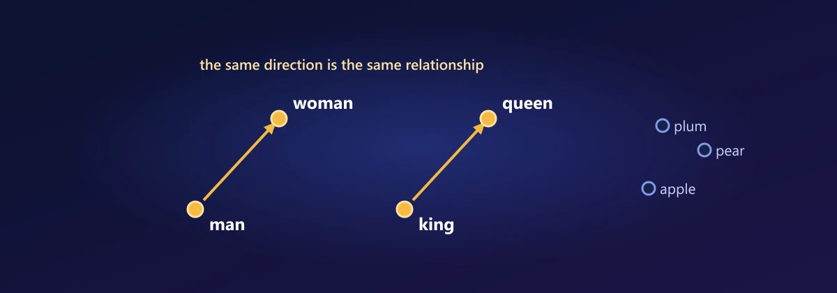
What you'll learn: how words become vectors whose geometry captures meaning, so that similar words sit close together and relationships become directions (king − man + woman lands near queen). We start by exploring pretrained word vectors, then build word vectors ourselves two ways: by counting and compressing, and by prediction with word2vec. Finally we see why one vector per word isn't enough, and how BERT gives every word a vector that depends on its sentence. The questions along the way lead into joint and marginal probabilities, pointwise mutual information, and the singular value decomposition.
Before you start: Lessons 1 to 10, especially vectors and cosine similarity (Lesson 2), probability distributions (Lessons 1, 3 and 4) and matrices (Lesson 5).
Explore pretrained word vectors
GloVe vectors were trained at Stanford on billions of words of Wikipedia and news text. Each of 400,000 words is a vector of 100 numbers. Load them (about 130 MB, once) and ask questions:
import gensim.downloader as api

glove = api.load("glove-wiki-gigaword-100")

print(glove.most_similar("coffee", topn=5))
print(glove.most_similar("python", topn=5))
print("cat ~ dog:", glove.similarity("cat", "dog"), "  cat ~ democracy:", glove.similarity("cat", "democracy"))

# Analogies: king - man + woman = ?
print(glove.most_similar(positive=["king", "woman"], negative=["man"], topn=3))
print(glove.most_similar(positive=["paris", "italy"], negative=["france"], topn=3))
print(glove.most_similar(positive=["walking", "swam"], negative=["walked"], topn=3))[('tea', 0.77326899766922), ('drinks', 0.7287518978118896), ('beer', 0.7253385186195374), ('cocoa', 0.7026589512825012), ('wine', 0.7002726793289185)]
[('monty', 0.6886237263679504), ('php', 0.586538553237915), ('perl', 0.5784407258033752), ('cleese', 0.5446676015853882), ('flipper', 0.5112984776496887)]
cat ~ dog: 0.8798075 cat ~ democracy: 0.0839781
[('queen', 0.7698540687561035), ('monarch', 0.6843381524085999), ('throne', 0.6755736470222473)]
[('rome', 0.8189547061920166), ('milan', 0.7376196980476379), ('naples', 0.7117615342140198)]
[('swimming', 0.7067671418190002), ('swim', 0.7048406600952148), ('biking', 0.6536761522293091)]Coffee sits next to other drinks, cat is far closer to dog than to democracy (and "python" lands between monty and cleese on one side and php and perl on the other, a clue we'll come back to), and simple arithmetic on vectors solves analogies: queen for king − man + woman, rome for paris − france + italy, swimming for walking − walked + swam. Nobody told the model about royalty, capitals or verb tenses. It worked them out from which words appear near which.
What just happened
Lesson 2 measured meaning with cosine similarity between sentence vectors. Here every word has its own vector, learned so that words used in similar contexts get similar vectors. The idea comes from linguistics. In 1957 J. R. Firth wrote: "You shall know a word by the company it keeps." In "I poured a cup of ___ and drank it hot", the blank is probably coffee or tea, not a bicycle. Coffee and tea appear in the same kinds of sentences, so they end up with similar vectors. This is the distributional hypothesis, and everything in this lesson is a way of turning it into numbers.
Why not just number the words?
Lesson 3 met this problem with cities. Numbering words (cat = 1, dog = 2, democracy = 3) imposes a false order. One-hot vectors (a 1 in the word's own position, zeros elsewhere) fix that, but every pair of one-hot vectors is equally far apart and perpendicular, so cat is exactly as similar to dog as to democracy. They're also as long as the vocabulary: 400,000 numbers, nearly all zero. We want short, dense vectors where distance means something. The first route there starts with counting.
What does it mean for words to keep company?
Question 1: how do we turn "appear near each other" into numbers?
Slide a window over a text and count how often each pair of words appears within a few words of each other. That gives a co-occurrence matrix, one row per word and one column per context word. Dividing the counts by their total turns them into probabilities. Here we use a tiny corpus of twelve sentences:
import numpy as np

corpus = """the king rules the kingdom
the queen rules the kingdom
the king is a man
the queen is a woman
the prince is a young man
the princess is a young woman
a man drinks coffee
a woman drinks tea
the dog chases the cat
the cat chases the mouse
a dog is an animal
a cat is an animal"""
sentences = [line.split() for line in corpus.split("\n")]
vocab = sorted({w for s in sentences for w in s})
idx = {w: i for i, w in enumerate(vocab)}
V, window = len(vocab), 2

pairs = [(idx[s[i]], idx[s[j]])
         for s in sentences for i in range(len(s))
         for j in range(max(0, i - window), min(len(s), i + window + 1)) if i != j]

counts = np.zeros((V, V))
for w, c in pairs:
    counts[w, c] += 1
print(V, "words,", len(pairs), "co-occurring pairs")
print("coffee appears near:", [vocab[c] for c in np.nonzero(counts[idx["coffee"]])[0]])21 words, 168 co-occurring pairs coffee appears near: ['drinks', 'man']
Two kinds of probability come out of this table. The joint probability P(w, c) is the chance that a randomly chosen pair is (w, c): its count divided by the total. The marginal probability P(w) is the chance that the first word of a random pair is w, whatever its partner: the row total divided by the total. Similarly P(c) uses the column totals.
When is a co-occurrence surprising?
Question 2: "the" appears next to almost every word. How do we separate meaningful company from mere frequency?
Ask how often two words appear together compared with how often they would if they had nothing to do with each other. If w and c were independent, the probability of seeing them together would be the product of their separate probabilities, P(w)·P(c); that is the definition of independence. Pointwise mutual information (PMI) compares the reality with that baseline, on a log scale:
Frequent words like "the" have large P(w), so the denominator cancels their sheer frequency. Rare pairs give unreliable negative values, so in practice negative PMI is clipped to zero, giving positive PMI (PPMI). Each row of the PPMI matrix is now a vector describing a word by its surprising company:
total = counts.sum()
P_wc = counts / total
P_w = counts.sum(axis=1) / total
P_c = counts.sum(axis=0) / total
with np.errstate(divide="ignore"):
    pmi = np.log(P_wc / np.outer(P_w, P_c))
ppmi = np.maximum(pmi, 0)

print("contexts of 'king', by raw count:")
for c in np.argsort(-counts[idx["king"]])[:4]:
print(f" {vocab[c]:8s} count {int(counts[idx['king'], c])} PPMI {ppmi[idx['king'], c]:.2f}")contexts of 'king', by raw count: the count 3 PPMI 1.10 a count 1 PPMI 0.24 rules count 1 PPMI 1.25 is count 1 PPMI 0.15
By raw count, "the" is king's most frequent companion, simply because "the" is everywhere. PPMI reorders them: "rules", which appears with king far more often than its overall frequency predicts, scores higher than "the" despite a third of the count, while "a" and "is", frequent everywhere, score near zero. On a real corpus of millions of sentences the effect is much stronger.
How do we squeeze a huge matrix into short vectors?
Question 3: each row has one entry per vocabulary word, so with 400,000 words the vectors are 400,000 long. How can we compress them to 100 numbers without losing the structure?
The tool is the singular value decomposition (SVD), one of the most useful facts in linear algebra. Every matrix, of any shape, can be written as a product of three simple ones:
In the language of Lesson 5, any linear map is a rotation, then a stretch along perpendicular axes, then another rotation. The singular values say how important each axis is. The Eckart-Young theorem says that keeping only the k largest singular values, with their columns of U and V, gives the best possible rank-k approximation of M: no other matrix built from k directions is closer, measured by the sum of squared differences. So the rows of U_k Σ_k are the best k-number summaries of the words' rows. We keep 5 dimensions instead of 21:
U, S, Vt = np.linalg.svd(ppmi)
print("singular values:", S[:8].round(2))
print("U Sigma V^T rebuilds the matrix:", np.allclose(U @ np.diag(S) @ Vt, ppmi))

k = 5
for rank in [2, 5, 10, V]:
    approx = U[:, :rank] @ np.diag(S[:rank]) @ Vt[:rank]
    print(f"rank {rank:2d}: approximation error {np.linalg.norm(ppmi - approx):.3f}")

E_svd = U[:, :k] * S[:k]                                  # one 5-number vector per word
E_svd /= np.linalg.norm(E_svd, axis=1, keepdims=True)     # unit length: dot = cosine

def neighbours(E, word, n=3):
    sims = E @ E[idx[word]]
    others = [i for i in np.argsort(-sims) if i != idx[word]]     # skip the word itself
    return [(vocab[i], round(float(sims[i]), 2)) for i in others[:n]]

for word in ["king", "dog", "coffee", "prince"]:
print(word, "->", neighbours(E_svd, word))singular values: [6.2 4.99 4.08 3.87 3.77 3.15 2.99 2.91]
U Sigma V^T rebuilds the matrix: True
rank 2: approximation error 10.244
rank 5: approximation error 7.689
rank 10: approximation error 4.379
rank 21: approximation error 0.000
king -> [('queen', 1.0), ('kingdom', 0.99), ('rules', 0.94)]
dog -> [('cat', 0.99), ('animal', 0.89), ('mouse', 0.88)]
coffee -> [('tea', 1.0), ('a', 0.94), ('young', 0.87)]
prince -> [('princess', 1.0), ('dog', 0.77), ('cat', 0.75)]The error shrinks as we keep more directions, and the 5-number vectors already place dog next to cat, coffee next to tea and prince next to princess. Counting, PMI and SVD are the classic recipe for word vectors, and GloVe is a refined version of it. The other route learns vectors by prediction.
Word2vec: learning by prediction
Word2vec (Mikolov and colleagues, 2013) trains a tiny model on a prediction task: for each word in the text (the centre word c), predict the words within a small window around it (the context words o). Every word gets two vectors: v_w when it is the centre and u_w when it is context. The probability of a context word is a softmax (Lesson 1) over the whole vocabulary:
The sum over the whole vocabulary is far too slow for millions of words. Negative sampling replaces it with a cheaper yes/no question: is this a real (centre, context) pair, or a fake one made with a random word? For each real pair it draws k random negative words, and maximises the log-probability of getting all these Bernoulli questions (Lesson 4) right:
Each term is the sigmoid-plus-cross-entropy pair from Lessons 4 and 7, so the gradient is again prediction minus label. Here is the whole algorithm in NumPy on the same toy corpus:
def sigmoid(z):
    return 1 / (1 + np.exp(-z))

rng = np.random.default_rng(0)
D = 10
W_in = rng.normal(0, 0.1, (V, D))      # centre vectors v: these become the embeddings
W_out = rng.normal(0, 0.1, (V, D))     # context vectors u
lr, k = 0.02, 3

for epoch in range(200):
    for c, o in pairs:
        negatives = rng.choice([w for w in range(V) if w != o], k, replace=False)
        ids = np.concatenate([[o], negatives])
        labels = np.array([1] + [0] * k)                  # 1 = real pair, 0 = fake
        v, U_ctx = W_in[c], W_out[ids]
        error = sigmoid(U_ctx @ v) - labels               # prediction minus label
        W_in[c] -= lr * error @ U_ctx
        W_out[ids] -= lr * np.outer(error, v)

E_w2v = W_in / np.linalg.norm(W_in, axis=1, keepdims=True)
for word in ["king", "man", "dog", "coffee", "prince"]:
print(word, "->", neighbours(E_w2v, word))king -> [('queen', 0.99), ('prince', 0.92), ('princess', 0.92)]
man -> [('woman', 0.96), ('tea', 0.67), ('coffee', 0.64)]
dog -> [('cat', 1.0), ('mouse', 0.85), ('prince', 0.82)]
coffee -> [('tea', 0.92), ('a', 0.76), ('young', 0.76)]
prince -> [('princess', 1.0), ('king', 0.92), ('queen', 0.89)]Two very different methods, counting-and-compressing and predicting, arrive at similar neighbourhoods. That's not a coincidence. In 2014 Omer Levy and Yoav Goldberg showed that skip-gram with negative sampling is, in effect, factorising a shifted PMI matrix: at the optimum, u_c · v_w ≈ PMI(w, c) − log k. Prediction and counting are two roads to the same geometry.
Why does vector arithmetic solve analogies?
Question 4: why should king − man + woman land near queen?
If the vectors capture which contexts each word prefers, then the difference between two words captures how their contexts differ. Man and woman appear in similar contexts except for gendered ones (he, she, his, her). King and queen differ in exactly the same way, since otherwise they both appear near crown, throne, rules. So king − man and queen − woman are approximately the same vector: a "royalty" offset. Rearranging, king − man + woman ≈ queen. In PMI terms, the offset reflects log-ratios of co-occurrence probabilities, which are consistent across many word pairs. The four words form an approximate parallelogram, which we can test directly:
royal_m = glove["king"] - glove["man"]
royal_f = glove["queen"] - glove["woman"]
cos = royal_m @ royal_f / (np.linalg.norm(royal_m) * np.linalg.norm(royal_f))
print("cosine between king-man and queen-woman:", round(float(cos), 3))
print("cosine between king-man and dog-cat:     ",
      round(float(royal_m @ (glove["dog"] - glove["cat"]) /
(np.linalg.norm(royal_m) * np.linalg.norm(glove["dog"] - glove["cat"]))), 3))cosine between king-man and queen-woman: 0.758 cosine between king-man and dog-cat: -0.187
The two offsets point in clearly similar directions; an unrelated offset doesn't. Analogies are far from perfect (most_similar also excludes the input words, which helps), but the parallelogram structure is real.
We can see it too. Project the vectors for six countries and their capitals onto the two directions along which they vary most (the top two singular vectors from Question 3), and draw an arrow from each country to its capital:
import matplotlib.pyplot as plt

pairs = [("france", "paris"), ("italy", "rome"), ("germany", "berlin"),
         ("japan", "tokyo"), ("china", "beijing"), ("russia", "moscow")]
words = [w for pair in pairs for w in pair]
X = np.array([glove[w] for w in words])
X = X - X.mean(axis=0)
_, _, Vt = np.linalg.svd(X, full_matrices=False)
P = X @ Vt[:2].T                                  # coordinates along the top two directions

plt.figure(figsize=(7, 5))
for i in range(0, len(words), 2):
    plt.annotate("", xy=P[i + 1], xytext=P[i], arrowprops=dict(arrowstyle="->", color="gray"))
plt.scatter(P[:, 0], P[:, 1])
for w, (x, y) in zip(words, P):
    plt.annotate(w, (x, y), textcoords="offset points", xytext=(5, 5))
plt.title("country to capital, GloVe vectors projected to 2D")
plt.show()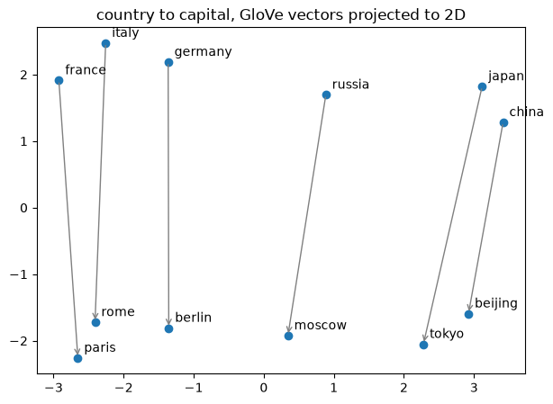
The six arrows are nearly parallel: going from a country to its capital is roughly the same move in every case. That shared direction is what the analogy arithmetic paris − france + italy ≈ rome relies on.
A warning: embeddings learn whatever patterns their training text contains, including society's biases. Early word2vec models completed "man is to computer programmer as woman is to ___" with "homemaker". Check for and mitigate such biases before using embeddings in decisions about people.
Embedding layers in neural networks
In a deep learning model, an embedding layer usually learns its vectors along with the rest of the network for the task at hand, as in Lesson 10's sentiment RNN. An embedding layer is just a lookup table: a matrix with one row per vocabulary word. Looking up row i is exactly multiplying a one-hot vector by that matrix: as Lesson 5 showed, multiplying by a basis vector simply picks out one row or column of a matrix. The lookup gives the same answer, only much faster:
import torch
from torch import nn

embedding = nn.Embedding(num_embeddings=V, embedding_dim=4)
word_id = idx["coffee"]
one_hot = torch.zeros(V)
one_hot[word_id] = 1
print(torch.allclose(embedding(torch.tensor(word_id)), one_hot @ embedding.weight))True
One vector per word is not enough
Question 5: "bank" means a riverside in one sentence and a financial institution in another. Which vector should it get?
A static embedding like GloVe or word2vec has to average all of a word's meanings into one vector, which represents none of them well: bank, bat, apple, spring, light. What we want is a vector for a word in its context. Contextual embedding models compute exactly that, from the whole sentence around the word. ELMo (2018) ran a bidirectional LSTM over the sentence; BERT (Google, 2018) used a transformer (Lesson 12) and became the standard.
BERT is pretrained by masked language modelling: hide 15% of the tokens and predict them from both sides. To fill in "I deposited cash at the [MASK]", the model must understand the whole sentence, so its internal vectors become context-aware representations of every token:
from transformers import AutoTokenizer, AutoModel

tokenizer = AutoTokenizer.from_pretrained("bert-base-uncased")
bert = AutoModel.from_pretrained("bert-base-uncased")

def word_vector(sentence, word):
    inputs = tokenizer(sentence, return_tensors="pt")
    with torch.no_grad():
        hidden = bert(**inputs).last_hidden_state[0]          # one 768-number vector per token
    tokens = tokenizer.convert_ids_to_tokens(inputs["input_ids"][0])
    return hidden[tokens.index(word)]

money_1 = word_vector("I deposited cash at the bank.", "bank")
money_2 = word_vector("The bank approved my loan.", "bank")
river = word_vector("We had a picnic on the river bank.", "bank")

cos = nn.functional.cosine_similarity
print("bank (money) vs bank (money):", round(cos(money_1, money_2, dim=0).item(), 3))
print("bank (money) vs bank (river):", round(cos(money_1, river, dim=0).item(), 3))bank (money) vs bank (money): 0.823 bank (money) vs bank (river): 0.522
The two financial uses of "bank" are more similar to each other than either is to the riverside bank, though the word is identical. With GloVe all three vectors would be the same. Contextual embeddings are what Lesson 2's sentence encoder builds on: it is a BERT-style model fine-tuned so that whole sentences with similar meanings get similar vectors.
Summary
Words become useful to neural networks as dense vectors whose geometry reflects meaning, following the distributional hypothesis: words in similar contexts have similar meanings. Counting co-occurrences gives joint and marginal probabilities; PMI, log P(w, c)/(P(w)P(c)), measures association beyond chance, with independence as the baseline. The SVD, M = UΣVᵀ, writes any matrix as rotate-stretch-rotate, and truncating it gives the best low-rank approximation, turning PPMI rows into short word vectors. Word2vec learns comparable vectors by predicting context words with negative sampling, which implicitly factorises a shifted PMI matrix. Consistent offsets make analogies work. An embedding layer is a lookup table, equivalent to one-hot times a matrix, and contextual models such as BERT give each occurrence of a word its own vector.
Exercises
1. Show that if w and c are independent, PMI(w, c) = 0. What is the largest possible PMI for a word pair that always appears together?
2. Compute the SVD of [[3, 0], [4, 5]] with NumPy. Check that the columns of U are unit length and perpendicular, and that UΣVᵀ rebuilds the matrix.
3. For a 100 × 100 random matrix, plot the approximation error of the rank-k SVD against k. Then do the same for the PPMI matrix of a larger corpus (a few paragraphs of a book). Why does the real-text curve fall faster?
4. Find three analogies that GloVe gets right and three it gets wrong. Can you explain the failures?
5. Train the NumPy word2vec with window sizes 1 and 4. How do the nearest neighbours change? Which window captures meaning, and which captures grammar?
6. Use BERT to compare the vectors for "bat" in a sentence about cricket and one about animals, and for "apple" as a fruit and a company.
Comments